How far can public summary PK data evaluate a change in the tarlatamab dosing interval?
A two-compartment model estimated from published aggregate PK values, comparing Q2W, Q3W and Q4W exposure in light of identifiability and uncertainty.
Key findings
- A two-compartment model fitted to six Cycle 2 PK summary values from the label explained them with a maximum error of 10.0%, but profiles showed CL, Q and Vp were poorly identified, and the terminal half-life (about 19.0 days) did not match the NCA median of 6.21 days.
- Extending the interval at the same 10 mg gives average-concentration ratios of 2/3 for Q3W and 1/2 for Q4W (fixed by mass balance under linear PK); the Q4W trough ratio was 0.371 with a wide conditional range of 0.171–0.498.
- The efficacy Emax relationship is based on first-cycle average concentration and cannot be reused as a threshold for maintenance troughs, and the per-dose fall in CRS cannot be explained by current exposure alone.
On this page
- Introduction
- 1. Background and questions
- 2. How to read the data
- 3. Mathematical model and estimation
- 4. Fit results and diagnostics
- 5. What changes when the interval is extended at the same 10 mg
- 6. Can this be linked to efficacy and CRS?
- 7. Answers to the QOI and the data needed next
- Reproducing the analysis
- References
Model estimation from public summary data, and exposure comparison that accounts for uncertainty
Introduction
If a mathematical model is built from published pharmacokinetic (PK) tables, concentrations under a different dosing interval can be calculated. But being able to draw a concentration curve is not the same as being able to use that prediction for a decision.
This article uses tarlatamab, a T-cell engager targeting DLL3, to estimate a two-compartment model from published PK summary values. Rather than simply entering published PopPK parameters, it fits the model to summary values derived from observations and examines what is determined by the data and what depends on assumptions.
In this analysis, the six summary values were explained within about 10%. However, uncertainty in clearance and peripheral distribution was large, and a wide range remained for trough concentrations when the interval was extended at the same dose. Relative changes in average concentration need to be evaluated separately from predictions of trough concentration.
1. Background and questions
For tarlatamab, the labeled regimen is 1 mg on the first day, 10 mg on Day 8, and 10 mg every 2 weeks from Day 15, each given intravenously over 1 hour.1 The initial step-up dosing and the subsequent maintenance dosing need to be treated as different questions.
Early on, the issues are the rise of exposure and the timing of CRS. In maintenance, the issue is how the maximum concentration, average exposure and the concentration just before the next dose change with the dosing interval. It is hard for a single PK metric to represent both.
The questions of interest (QOI) are:
- Can the public PK summary values be explained with a two-compartment model, and how well can its four parameters be identified?
- If the same 10 mg is given Q2W, Q3W or Q4W, how do the steady-state maximum, average and trough concentrations change?
- Can that exposure difference be interpreted all the way to the published efficacy and CRS information?
The context of use (COU) is model reconstruction and scenario comparison based on public information for research and learning. It is not used for individual dose adjustment, changing the approved regimen, or guaranteeing the efficacy or safety of Q3W or Q4W.
2. How to read the data
The main analysis used six values — maximum concentration, AUC and pre-dose concentration — from the Cycle 2 Day 1 and Day 15 PK table in the PMDA package insert.1 The "Ctrough" in that table is explicitly labeled "pre-dose concentration" in the corresponding Table 23 of the review report.2 In this analysis it was therefore matched to the time just before the dose on that day. Replacing it with the concentration 14 days after a dose would misalign the time points of the fit.
| Time point | Metric | Geometric mean (CV%) | n | Unit |
|---|---|---|---|---|
| Cycle 2 Day 1 | Pre-dose concentration | 0.288 (48) | 16 | µg/mL |
| Cycle 2 Day 1 | Cmax | 2.8 (38) | 19 | µg/mL |
| Cycle 2 Day 1 | AUC0–336h | 242 (41) | 18 | h·µg/mL |
| Cycle 2 Day 15 | Pre-dose concentration | 0.309 (47) | 12 | µg/mL |
| Cycle 2 Day 15 | Cmax | 2.65 (41) | 18 | µg/mL |
| Cycle 2 Day 15 | AUC0–336h | 298 (48) | 15 | h·µg/mL |
Concentrations and AUCs are geometric means with CV% in parentheses. The number of patients differs by metric. The half-life of 6.21 days is a median reported for Cycle 2 Day 15, a different statistic from the geometric-mean PK metrics.1 Here the half-life was not included in the fit and was used only as an interpretive check.
These are not individual patients' concentrations. The correspondence between metrics from the same patient, dose delays, covariates and details of missing data are not available. The published population PK analysis used 420 patients and 8,509 samples; the information used here is six summary values.3 This is not described as a reproduction of the original NLME analysis.
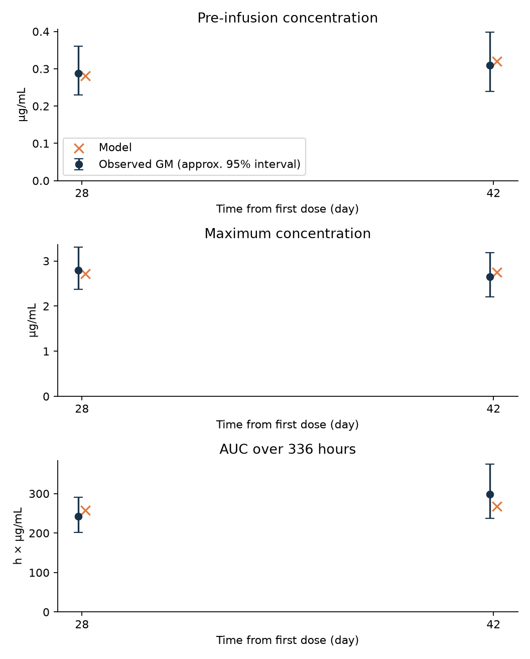
Figure 1. Points are public geometric means and crosses are model predictions. Error bars are 95% intervals for the geometric mean approximated on the log scale from the reported CV and number of patients, not the 95% range between patients. AUC, which has different units, is not overlaid on the same axis as concentrations.
3. Mathematical model and estimation
Let \(A_c\) and \(A_p\) be the drug amounts in the central and peripheral compartments. A two-compartment model with linear elimination was used.
\[ \begin{aligned} \frac{dA_c}{dt}&=R_{\mathrm{in}}(t)-\frac{CL+Q}{V_c}A_c+\frac{Q}{V_p}A_p,\\ \frac{dA_p}{dt}&=\frac{Q}{V_c}A_c-\frac{Q}{V_p}A_p. \end{aligned} \]
\[ \begin{aligned} C(t)&=\frac{A_c(t)}{V_c},\\ R_{\mathrm{in}}(t)&=\frac{D}{T_{\mathrm{inf}}},\\ T_{\mathrm{inf}}&=\frac{1}{24}\ \mathrm{day}. \end{aligned} \]
The input rate applies only during the infusion and is 0 otherwise. Time is in days, drug amount in mg and volume in L, so \(C(t)\) in mg/L is numerically equal to µg/mL. AUC was converted from days to hours for comparison with the published values.
The first dose is at \(t=0\), with doses at 0, 7, 14, 28 and 42 days. Cycle 2 Day 1 and Day 15 correspond to days 28 and 42. The pre-dose concentration is calculated before the new dose is added, the maximum concentration at the end of the infusion, and AUC as the integral over the 14 days after that dose. A planned dosing history without delays or interruptions is assumed.
Because the system is a fixed linear system, the state was updated with matrix exponentials for each interval. A separate numerical integrator, solve_ivp, was used to check the implementation. At the estimated parameters, the difference in drug amount was 8.6e-13 mg and the difference in AUC was 2.9e-12 µg·day/mL; numerical differences are far too small to explain the estimation results below.
Objective function for summary values
The reported CV was converted to a proportion, and the log-scale standard error of the geometric mean was approximated as
\[ s_j=\sqrt{\frac{\log(1+CV_j^2)}{n_j}}. \]
Parameters were estimated on the log scale by minimizing the weighted sum of squared log residuals.
\[ J(\theta)=\sum_j\left\{\frac{\log Y_j^{\mathrm{model}}(\theta)-\log Y_j^{\mathrm{obs}}}{s_j}\right\}^{2}. \]
\[ \theta=(CL,V_c,V_p,Q). \]
This is a working approximation that treats the error of each summary value as an independent normal distribution. Cmax and AUC calculated from the same patients may be correlated, but that covariance is not published. Also, the geometric mean of a population generally does not equal the value calculated from a single representative parameter set. What is estimated here is a representative model that approximates the summary values, not the typical parameters or IIV of the population.
The values used for external comparison are \(CL=0.649\) L/day, \(V_c=3.44\) L, \(V_p=5.06\) L and \(Q=1.11\) L/day.4 They were neither fixed nor added to the objective function as a penalty.
4. Fit results and diagnostics
| Parameter | Estimate here | Public PopPK value (for comparison) | Unit |
|---|---|---|---|
| CL | 0.845 | 0.649 | L/day |
| Vc | 4.075 | 3.44 | L |
| Vp | 10.162 | 5.06 | L |
| Q | 0.792 | 1.11 | L/day |
The maximum absolute relative error against the public summary values was 10.0%.
| Time point | Metric | Public value | Model prediction | Relative error | Unit |
|---|---|---|---|---|---|
| C2D1 | Pre-dose concentration | 0.288 | 0.281 | -2.6% | µg/mL |
| C2D1 | Cmax | 2.8 | 2.714 | -3.1% | µg/mL |
| C2D1 | AUC0–336h | 242 | 257.800 | +6.5% | h·µg/mL |
| C2D15 | Pre-dose concentration | 0.309 | 0.321 | +3.7% | µg/mL |
| C2D15 | Cmax | 2.65 | 2.754 | +3.9% | µg/mL |
| C2D15 | AUC0–336h | 298 | 268.342 | -10.0% | h·µg/mL |
Optimization from 30 different starting values was judged successful in every case and reached the same minimum objective function. The objective function was 16.49 for one compartment and 1.70 for two compartments. The fit to these summary values improved with two compartments, but four parameters are being fitted to six values, and independent errors are assumed, so this difference alone does not settle the model structure.
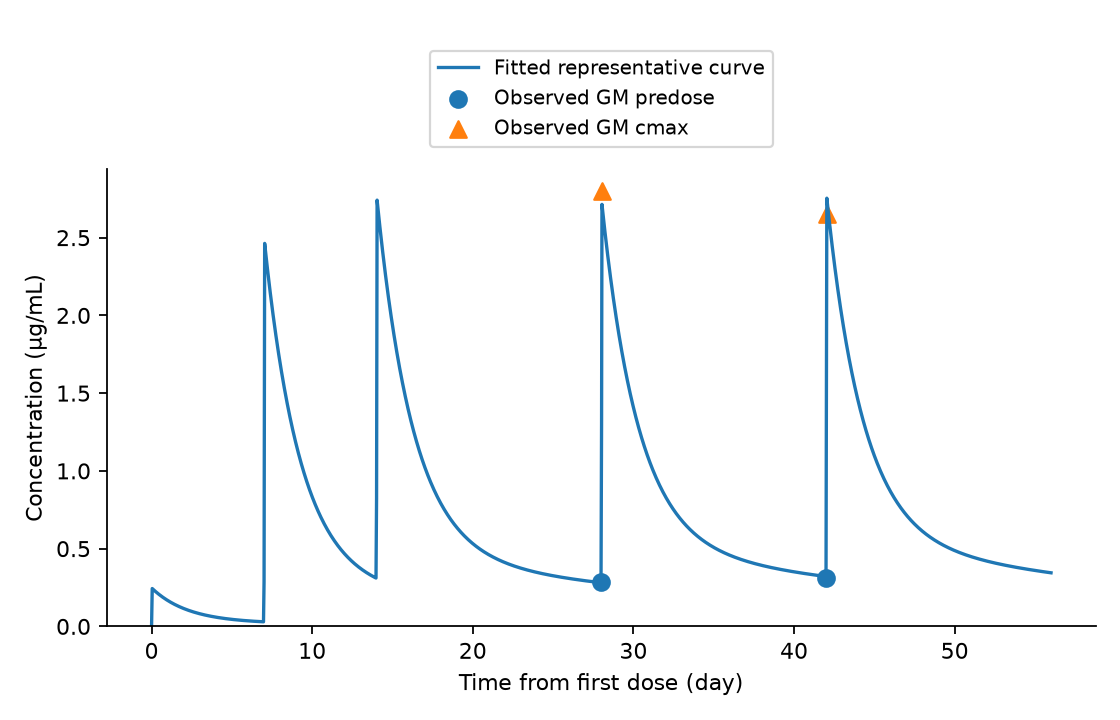
Figure 2. The line is a representative curve calculated from the estimated model. Only the Cycle 2 summary values for pre-dose and maximum concentration are overlaid as observations; there are no observed data at the many time points along the line. The mean concentration curves in published figures were not digitized here.
Convergence of the optimization and identifiability are different problems
A profile analysis was performed in which each parameter was fixed and the rest were re-optimized.
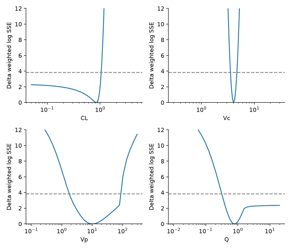
Figure 3. The horizontal axis is on a log scale. The dashed line at 3.84 is a reference value often used for a likelihood ratio with one degree of freedom; under the present approximation, small sample and search bounds, it does not guarantee an exact 95% interval. The vertical axis is limited to 0–12.
Vc has a relatively sharp minimum. For CL toward lower values and for Q toward higher values, however, the objective function does not increase enough. A wide range also remains for Vp. Even though the optimization is stable, the parameters are not strongly determined by the data.
The terminal half-life of the estimated model was about 19.0 days, not the same as the public NCA median of 6.21 days. The NCA observation window, the population summary statistic and the long-term asymptotic phase of the model do not measure the same thing, so it is not appropriate either to reject the model on this difference alone or to ignore the mismatching half-lives. The terminal phase is not treated as sufficiently identified by these summary values.
Hold-out is not external validation
The three values for one of the Cycle 2 dosing days were removed, and the four parameters were re-estimated from the remaining three values only.
| Time point removed | Metric | Prediction error |
|---|---|---|
| C2D1 | Pre-dose concentration | -4.2% |
| C2D1 | Cmax | -6.5% |
| C2D1 | AUC0–336h | +19.3% |
| C2D15 | Pre-dose concentration | +6.8% |
| C2D15 | Cmax | +7.2% |
| C2D15 | AUC0–336h | -15.1% |
The prediction error for AUC widened to about 15–19%. This is a diagnostic of instability when information is reduced. Because the number of training values is below the number of parameters and the result depends on how the optimum is chosen, it is not called validation of predictive performance in independent patients or trials.
5. What changes when the interval is extended at the same 10 mg
Q2W, Q3W and Q4W were compared as intervals of 14, 21 and 28 days. Each dose is 10 mg, so dose intensity is not maintained. Steady state was calculated directly from the condition that drug amounts return to the same state after one cycle, rather than approximated with many doses.
| Regimen | Cmax (µg/mL) | Cavg (µg/mL) | Ctrough (µg/mL) | Cmax ratio | Cavg ratio | Ctrough ratio |
|---|---|---|---|---|---|---|
| 10 mg Q2W | 2.814 | 0.846 | 0.381 | 1.000 | 1.000 | 1.000 |
| 10 mg Q3W | 2.651 | 0.564 | 0.218 | 0.942 | 0.667 | 0.573 |
| 10 mg Q4W | 2.575 | 0.423 | 0.141 | 0.915 | 0.500 | 0.371 |
Concentrations are in µg/mL and ratios are relative to 10 mg Q2W. The table gives point estimates for the representative model, not predictions for individual patients.
With linear PK, mass balance over one cycle gives
\[ C_{\mathrm{avg}}^{ss}=\frac{D}{CL\tau}. \]
For a relative comparison at the same dose and the same patient's CL,
\[ \begin{aligned} \frac{C_{\mathrm{avg,Q3W}}^{ss}}{C_{\mathrm{avg,Q2W}}^{ss}}&=\frac{14}{21}=\frac{2}{3},\\ \frac{C_{\mathrm{avg,Q4W}}^{ss}}{C_{\mathrm{avg,Q2W}}^{ss}}&=\frac{14}{28}=\frac{1}{2}. \end{aligned} \]
These ratios do not change even if Vp and Q are uncertain. The absolute average concentration, however, still carries the uncertainty in CL. What is stable is the ratio due to the interval, assuming linear, time-invariant CL.
Propagating uncertainty to predictions
Summary values were generated around the six fitted predictions using the log-scale standard errors above, and the model was re-estimated 300 times. This is neither patient resampling nor IIV estimation; it is a summary-level parametric bootstrap that assumes independent summary errors and a fixed model.
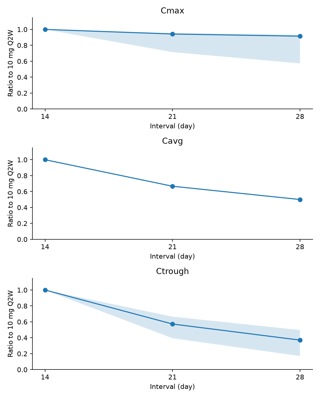
Figure 4. The bands are conditional widths with the structural model, dosing history, independent errors and parameter search range held fixed. They are not 95% prediction intervals for a future patient population. The band for the Cavg ratio coincides with the line because, by the mass balance above, the ratio is fixed algebraically.
| Regimen | Metric | Point estimate of ratio | Conditional 2.5–97.5% range |
|---|---|---|---|
| 10 mg Q3W | Cmax | 0.942 | 0.715–0.954 |
| 10 mg Q3W | Ctrough | 0.573 | 0.395–0.665 |
| 10 mg Q4W | Cmax | 0.915 | 0.573–0.934 |
| 10 mg Q4W | Ctrough | 0.371 | 0.171–0.498 |
The search range was CL 0.05–5 L/day, Vc 0.3–30 L, Vp 0.1–300 L and Q 0.01–20 L/day. Of the 300 replicates, CL reached the lower bound in 6.3% and Q reached the upper bound in 4.0%. Replicates that reached a bound were not excluded from the summary, but these widths are limited by the search bounds. They should not be carried into clinical decisions as "95% confidence intervals".
A sensitivity analysis was also performed assuming a common correlation among the three metrics on the same dosing day.
| Assumed correlation between metrics | CL | Vc | Vp | Q | Q4W/Q2W trough ratio |
|---|---|---|---|---|---|
| 0 | 0.845 | 4.075 | 10.162 | 0.792 | 0.371 |
| 0.5 | 0.872 | 4.090 | 8.664 | 0.764 | 0.352 |
| 0.8 | 0.899 | 4.137 | 7.787 | 0.755 | 0.338 |
The correlations of 0.5 and 0.8 are not measured estimates but assumptions for examining the effect of the missing covariance. The correlation between dosing days is set to 0 in this sensitivity analysis as well. The data here alone still cannot select an appropriate correlation structure.
Comparisons that maintain average exposure ask a different question
So far the dose per administration has been fixed at 10 mg. As a different question, hypothetical scenarios that keep the dose intensity \(D/\tau\) were also calculated. Relative to 10 mg Q2W, 15 mg Q3W and 20 mg Q4W give equal average exposure under linear PK.
| Hypothetical regimen | Cmax ratio | Cavg ratio | Ctrough ratio |
|---|---|---|---|
| 10 mg Q2W | 1.000 | 1.000 | 1.000 |
| 15 mg Q3W | 1.413 | 1.000 | 0.859 |
| 20 mg Q4W | 1.830 | 1.000 | 0.741 |
All values are ratios for the representative model relative to 10 mg Q2W. The 15 and 20 mg schedules are assumptions for comparison, not approved regimens or dose proposals.
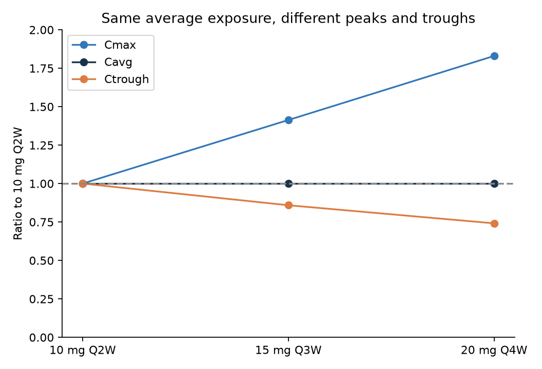
Figure 5. A structural comparison based on the parameter point estimates. Even with the same average exposure, extending the interval raises the maximum concentration and lowers the trough. Bootstrap widths are not shown in this figure, and the peak and trough ratios carry the same estimation limitations as in Figure 4.
In other words, when evaluating "extending the dosing interval", it must first be decided whether the dose per administration is fixed or average exposure is maintained. The ability to maintain average exposure alone does not show that safety related to peaks, or efficacy late in the interval, is also maintained. Stating the conditions of a regimen comparison is itself the first step toward using a model for decisions.
6. Can this be linked to efficacy and CRS?
Which exposure metric is the efficacy "plateau" about?
The DCR Emax relationship in the FDA document uses the first-cycle average concentration as the explanatory variable, with \(E_{\max}=0.650\) and \(EC_{50}=49.4\) ng/mL.4
\[ P(\mathrm{DCR})=E_{\max}\frac{E}{EC_{50}+E}. \]
In this equation, the exposures corresponding to 90% and 95% of the maximal effect are \(9EC_{50}=444.6\) ng/mL and \(19EC_{50}=938.6\) ng/mL. This does not mean DCR is 90% or 95%.
Also, \(E\) here is the average concentration in the first cycle. This threshold cannot be applied directly to maintenance Ctrough to conclude that "Q4W is effective because the threshold is exceeded". The published E–R analysis and this summary PK analysis differ in population, exposure metric and estimation method.5 Sharing the same unit does not make the explanatory variables interchangeable.
Do not explain the fall in CRS by current exposure alone
In the 10 mg cohort of DeLLphi-301, the numbers of patients reporting CRS in the periods after the first, Day 8 and Day 15 doses were 54/133, 39/133 and 10/133.6 The early incidence is high even though the first dose is small.
From this summary, it is hard to explain the differences between doses with a single-variable relationship in which "higher blood concentration means more CRS". Nor can the fall in incidence be taken as proof of a mechanism of immune adaptation, because premedication, management, dosing history, patient status and the handling of recurrence in the same patients cannot be separated.
This article does not fit a new CRS model that treats the three per-dose summaries as independent patient data. Presenting a hypothesis from summary points was kept distinct from predicting risk based on each patient's exposure and onset time. Links to E–R and CRS are limited to interpreting public information and organizing the data needed.
7. Answers to the QOI and the data needed next
| Question | What can be supported here | What cannot be supported |
|---|---|---|
| Can the public PK be explained? | A representative model explained the six summary values within about 10% | Recovering the original PopPK parameters and IIV, or reproducing individual concentrations |
| What is the effect of the interval? | Under linear PK, the average-concentration ratio is 2/3 for Q3W and 1/2 for Q4W | Using absolute concentrations or troughs as precise patient predictions |
| Can this be linked to efficacy and CRS? | Showed the need to separate exposure metrics and dosing history | Guaranteeing maintained efficacy or reduced CRS with Q3W or Q4W |
The follow-up questions concern maintenance troughs, peak safety after dose increases, and early CRS. Each requires different measurements.
| Next question | Metric to evaluate | Additional information needed |
|---|---|---|
| Can exposure late in the interval be maintained? | Maintenance Ctrough and its uncertainty | Dosing records for the same patients, several concentrations late in the interval, information on missing data and delays |
| Does the peak become a problem with dose increases that keep average exposure? | Cmax and corresponding safety | Concentrations at the end of infusion and in the distribution phase; adverse events and their times by patient |
| What are the early CRS differences linked to? | Exposure and onset time after each dose | Within-patient correspondence including dose number, premedication, recurrence and patient status |
Adding the covariance between PK metrics would also allow the currently assumed error structure to be updated. Conversely, drawing the curves more precisely without this information does not resolve the uncertainty needed for decisions.
If published concentration curves are digitized, the type of mean, the number of patients at each time point, the error bars and the reading error need to be recorded before adding them to the model. It should not be assumed that adding curves improves the identifiability of Vp or Q; the profile analysis and prediction widths should be checked again.
In this analysis, the constraint was the definition and information content of the summary values rather than numerical accuracy: which time point the pre-dose concentration corresponds to, whether average concentration and trough are distinguished, and whether uncertainty is propagated to predictions. These checks need to be done before linking the model to a use.
Reproducing the analysis
Download the analysis code, input CSV and result tables. The random seed is 20261003. Estimation, the 30-start optimization, profiles, the 300-replicate bootstrap, hold-out, the covariance sensitivity analysis and the comparison with an independent ODE implementation run from one script. No patient-level data are included.
In the folder where the ZIP is extracted, run the following. The input is data/observations.csv, and outputs are saved in results/ and figures/.
python -m pip install -r requirements.txt
python analysis.py
References
- PMDA. Imdelltra package insert, 16.1.1, Table 1 (Japanese). Revised May 2026; accessed 2026-10-03.
- PMDA. Imdelltra review report, Table 23 (PDF page 24; Japanese). 2024-12-27.
- Kong S, et al. Population Pharmacokinetics of Tarlatamab. Clin Pharmacokinet. 2025;64:729–741.
- FDA. Tarlatamab Multidisciplinary Review, Tables 66 and 71. 2024.
- Chen PW, et al. Tarlatamab Exposure–Efficacy and Exposure–Safety Relationships to Inform Dose Selection. Clin Cancer Res. 2025;31:4688–4697.
- Sands JM, et al. Practical management of adverse events in patients receiving tarlatamab. Cancer. 2025;131:e35738, Figure 2.
Cite this article
Kumakura, D. (2026). How far can public summary PK data evaluate a change in the tarlatamab dosing interval?. daikikumakura.github.io. https://daikikumakura.github.io/writing/tarlatamab-summary-pk-en.html