Can matching average exposure alone set the tarlatamab dosing interval?
Between-subject variability simulated from a published population PK model, with efficacy exposure–response, period-specific CRS and maintenance exposure examined separately. Matching average exposure does not preserve peaks and troughs, and the analysis shows the limits of deciding from public information.
Key findings
- Recalculating the published PopPK model (FDA Tables 66–67) in 5,000 virtual subjects matched initial-dose exposure to the label means, but the steady-state trough was about 16–41% higher, so population exposure is not fully reproduced.
- Matching dose intensity to 10 mg Q2W does not preserve the profile: 20 mg Q4W kept average exposure but gave a median peak of about 1.78× and a median trough of about 0.60×.
- Efficacy saturation (Cycle 1 Cavg), CRS by period and low maintenance concentrations need separate evidence; matching average exposure alone cannot establish equivalence of maintenance regimens.
On this page
- Background and questions
- Data and the type of evidence
- Reproducing the public PopPK model
- How to read the efficacy exposure–response
- Can CRS be summarized as "lower concentration, less CRS"?
- Maintenance: the same average exposure, a different profile
- What to examine next
- Conclusion
- Reproducing the analysis
- References
I reproduced the published population PK (PopPK) model of tarlatamab and examined four things separately: initial dosing, efficacy exposure–response, the timing of cytokine release syndrome (CRS), and maintenance exposure. What public information supports most easily is a comparison of PK under different dosing conditions. Linking those comparisons to efficacy or CRS requires checking that the exposure metric and observation period match the original analyses.
In this analysis, extending the dosing interval while increasing the dose proportionally preserved average exposure but not peaks or troughs. This difference shows that matching average exposure alone cannot establish equivalence of maintenance regimens. What follows is a research and learning reanalysis of public documents and is not to be used for treatment or for dose decisions in clinical trials.
Background and questions
Tarlatamab is a T-cell engager targeting DLL3 and CD3. The US label regimen is 1 mg on Day 1, 10 mg on Days 8 and 15, then 10 mg every 2 weeks, each as a 1-hour intravenous infusion.[1] The initial step-up and the subsequent maintenance phase raise different questions.
| Question (QOI) | Metric used here | Scope of the judgment |
|---|---|---|
| Is the recalculation of the public model sound? | Cavg, Cmax and Ctrough after the first dose, the first 10 mg dose and at steady state | Implementation consistency and differences from published summaries |
| What does "efficacy saturates" mean? | Cycle 1 Cavg and the published Emax model | Interpretation and scope of average exposure |
| How is CRS distributed across doses? | Number of patients with all-grade CRS by observation period | What the summary does and does not show |
| What changes when the maintenance interval is extended? | Steady-state average, peak and trough; within-patient ratios | PK trade-offs |
The context of use (COU) is the comparison of exposure between regimens using the public tarlatamab model. Transferring mg doses to new DLL3-targeted drugs, predicting risk for individual patients, and guaranteeing the efficacy or safety of Q3W/Q4W are out of scope.
Data and the type of evidence
| Source | Information used | Type of evidence |
|---|---|---|
| FDA multidisciplinary review (2024), Tables 66–67 | Two-compartment PK, IIV, intervals for fixed effects | Published model estimates[2] |
| Original PopPK paper (2025) | 420 patients, 8,509 samples, model and role of covariates | Original analysis of patient data[3] |
| Original exposure–response paper (2025), FDA Table 71 | Efficacy model against Cycle 1 Cavg | Published exposure–response estimates[2,4] |
| DeLLphi-301 adverse-event management paper, Figure 2 | CRS counts by period in 133 patients | Published observational summary[5] |
| US label, Section 12.3, Table 17 | Mean concentrations with CV%, dosing conditions | Model-based published summaries[1] |
Individual concentrations, actual dosing times, CRS onset times and their link to premedication or tumor burden were not available. The 5,000 subjects here are virtual subjects generated from the model's between-subject variability, not clinical data. Recalculating a published model is also a different task from NLME estimation with new patient data; the latter was not done here.
The documents were checked on 3 October 2026. Because observation and management conditions on the label can be updated, the historical CRS summary of 133 patients is not mixed with current safety summaries. This article does not describe dosing or management procedures.
Reproducing the public PopPK model
Model and units
With drug amounts \(A_c, A_p\) (mg) in the central and peripheral compartments,
\[ \frac{dA_c}{dt}=R_{in}(t)-\frac{CL+Q}{V_c}A_c+\frac{Q}{V_p}A_p, \qquad \frac{dA_p}{dt}=\frac{Q}{V_c}A_c-\frac{Q}{V_p}A_p. \]
Concentration is \(C=A_c/V_c\). Time is in days and flow in L/day. Computed mg/L were multiplied by 1,000 to give ng/mL. The 1-hour infusion was implemented as a constant-rate input over a finite time, not as an instantaneous bolus.
| Parameter | Reference value | Published 95% CI |
|---|---|---|
| CL (L/day) | 0.649 | 0.616–0.682 |
| Vc (L) | 3.44 | 3.25–3.62 |
| Q (L/day) | 1.11 | 0.874–1.34 |
| Vp (L) | 5.06 | 4.40–5.71 |
| SD of η for CL | 0.437 | 0.364–0.510 |
| SD of η for Vc | 0.387 | 0.329–0.445 |
| Correlation of ηCL and ηVc | 0.535 | 0.314–0.755 |
Source: FDA Tables 66–67.[2] The IIV values 0.437 and 0.387 are used as standard deviations and a correlation, as presented in that table. They are not interpreted as CVs and converted back to log-SDs.
\[ CL_i=0.649\exp(\eta_{CL,i}),\quad V_{c,i}=3.44\exp(\eta_{Vc,i}),\quad \begin{pmatrix}\eta_{CL,i}\\\eta_{Vc,i}\end{pmatrix} \sim N\left(0,\begin{pmatrix} 0.437^2&0.535(0.437)(0.387)\\ 0.535(0.437)(0.387)&0.387^2 \end{pmatrix}\right). \]
Five thousand subjects were generated with the fixed seed 20261005. All were fixed at the reference covariates (73 kg, White, binding ADA negative), and Q and Vp were fixed. This is not a regeneration of the trial population with the original covariate model for body weight, race and ADA. Residual error is error in observations and was not added to the distribution of latent exposure.
The comparison was paired: every virtual subject received every regimen. This separates between-subject differences from changes due to the regimen better than comparing two independently generated populations.
What was verified
The analytical solution was checked against an independent matrix-exponential solution, and the total AUC after a single dose converged to Dose/CL. At steady state \(C_{avg,ss}=Dose/(CL\tau)\) is used. These are checks of the implementation and do not replace validation of clinical predictive performance.
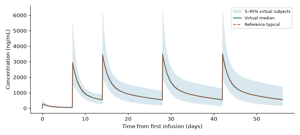
Values are in ng/mL. The published value is the label mean, the typical value uses η = 0, and the virtual mean is the arithmetic mean of the population fixed at the reference covariates.
| Period | Metric | Published mean | Typical value | Virtual mean |
|---|---|---|---|---|
| First 1 mg dose, 7 days | Cavg | 106 | 106.6 | 106.8 |
| Same | Cmax | 314 | 287.6 | 311.6 |
| Same | Ctrough | 49 | 51.0 | 51.8 |
| First 10 mg dose, 7 days | Cavg | 1,100 | 1,106.4 | 1,109.4 |
| Same | Cmax | 3,190 | 2,927.1 | 3,168.0 |
| Same | Ctrough | 517 | 541.8 | 552.2 |
| Steady state 10 mg Q2W | Cavg | 1,040 | 1,100.6 | 1,216.3 |
| Same | Cmax | 3,640 | 3,423.1 | 3,779.0 |
| Same | Ctrough | 472 | 548.2 | 664.2 |
The virtual mean brings the initial peaks close to the published means. The steady-state trough, however, does not match: it is about 16% higher than the published mean for the typical value and about 41% higher for the virtual mean. Because the covariate distribution of the population and differences in the model and summarization method were not reproduced, not every metric can be said to match.
The implementation is therefore consistent as a calculation from the public reference parameters, but it is not treated as a model that fully reproduces the population exposure on the label. The comparisons below are mainly relative changes within the same model and the same subjects. They are not used to judge absolute trough thresholds.
How to read the efficacy exposure–response
The published analysis uses the model-estimated Cycle 1 average concentration as the explanatory variable, not the dose itself.[4]
\[ p(E)=\frac{E_{max}E}{EC_{50}+E},\qquad E=C_{avg,\mathrm{first\ cycle}}. \]
The formal estimates were confirmed in the publisher's Supplementary Table S1.[4] For ORR, \(E_{max}=0.339\) and \(EC_{50}=57.4\) ng/mL (95% CI 22.5–146); for DCR, \(E_{max}=0.650\) and \(EC_{50}=49.4\) ng/mL (95% CI 20.9–117). No new Emax estimation is attempted without patient-level data.
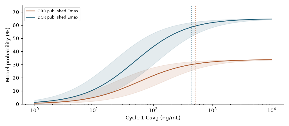
\(E_{90}=9EC_{50}=444.6\) ng/mL is the Cycle 1 Cavg that reaches 90% of the model maximum. It is not the concentration at which DCR reaches 90%; in this model it corresponds to \(0.9\times0.650=58.5\%\). There is also no basis for converting it into a Ctrough threshold for maintenance dosing.
The predictions reported in the original paper are shown separately from the recalculated values.[4]
| Target dose Q2W | Published predicted ORR | Published predicted DCR |
|---|---|---|
| 3 mg | 26.2% | 52.0% |
| 10 mg | 31.4% | 60.8% |
| 100 mg | 33.6% | 64.5% |
These are predictions of the original model evaluated at the median exposure for each dose, not observed response rates and not mean response rates in this virtual population. In a nonlinear model, \(p(\operatorname{mean}E)\) and \(\operatorname{mean}p(E)\) generally differ.
The ORR EC50 could not be confirmed from the text extracted from the FDA document, but it was confirmed as 57.4 ng/mL in the publisher's supplementary PDF. This formal estimate was used instead of back-calculating from the three published predictions. The ORR \(E_{90}\) is 516.6 ng/mL. The EC50 intervals of both models are wide, so the approximate saturation point is not treated as a precise threshold.
Saturation near 10 mg is consistent with the published interpretation that higher doses add little benefit. It does not, however, demonstrate equivalence of other schedules that produce the same Cycle 1 average exposure. Still less can this concentration or mg dose be transferred directly to another DLL3-targeted drug, which differs in binding, half-life, distribution and mechanism.
Can CRS be summarized as "lower concentration, less CRS"?
For the 133 patients in DeLLphi-301, the period-specific summary in Figure 2 was used.[5] These are all-grade CRS counts and should not be confused with grade ≥2 or ≥3. Wilson 95% intervals were recalculated for each period.
| Observation period | Patients with CRS / 133 | Proportion | Wilson 95% interval |
|---|---|---|---|
| C1D1–7 | 54 | 40.6% | 32.6–49.1% |
| C1D8–14 | 39 | 29.3% | 22.2–37.6% |
| C1D15–28 | 10 | 7.5% | 4.1–13.3% |
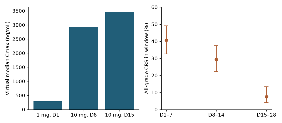
In the reference model, the peak rises when the dose is stepped up from 1 mg to 10 mg, and it rises again with the next 10 mg dose because of residual drug. The period-specific CRS proportions in the clinical summary, by contrast, decrease. This is a reason to examine dosing history and observation conditions before describing the whole course with a single monotonically increasing concentration–CRS relationship.
However, this opposite direction alone cannot prove biological adaptation. The same patients appear in several periods, and the last period lasts 14 days compared with 7 days for the first two. The risk set for each actual dose, premedication, changes in tumor burden, discontinuations and delays, and CRS recurrence are not known patient by patient.
The three periods are therefore not tested as three independent groups, and no tolerance or adaptation parameters are estimated from three points. Nor can 54 + 39 + 10 be summed as "the number of patients who experienced CRS". Figure 2 is a period-by-period descriptive summary, not a model that gives the CRS probability of an individual's next dose.
Maintenance: the same average exposure, a different profile
The comparator is steady-state 10 mg Q2W. Using the same CL and Vc for each virtual subject, four conditions were compared:
- 10 mg Q3W and 10 mg Q4W: the dose per administration is fixed and the interval is extended.
- 15 mg Q3W and 20 mg Q4W: the dose per unit time is matched to 10 mg Q2W.
These are computational counterfactuals, not recommended regimens. Ratios are formed by dividing each subject's metric by that subject's own 10 mg Q2W value and then summarized.
| Condition | Cavg ratio | Cmax ratio [5–95%] | Ctrough ratio [5–95%] |
|---|---|---|---|
| 10 mg Q2W | 1.000 | 1.000 | 1.000 |
| 10 mg Q3W | 0.667 | 0.923 [0.857–0.966] | 0.518 [0.434–0.580] |
| 10 mg Q4W | 0.500 | 0.888 [0.789–0.952] | 0.298 [0.206–0.377] |
| 15 mg Q3W | 1.000 | 1.385 [1.286–1.450] | 0.778 [0.651–0.870] |
| 20 mg Q4W | 1.000 | 1.776 [1.579–1.905] | 0.597 [0.412–0.753] |
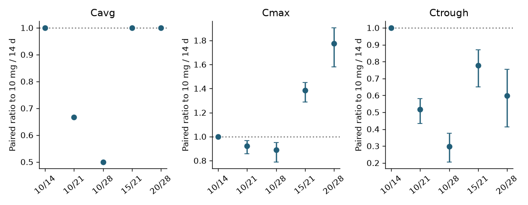
With the dose per administration fixed, average exposure and trough fall. When dose intensity is matched, average exposure is mathematically equal for any CL, but the peak rises and the trough falls. For Q4W, even with the average preserved, the median peak was about 1.78 times and the median trough about 0.60 times that of 10 mg Q2W.
This shows that a comparison matched on average exposure narrows the question. A finding that efficacy is associated with average exposure is not the same as a finding that periods of low concentration are acceptable. Nor can safety necessarily be judged with the same exposure metric as efficacy.
Separating between-subject variability from estimation uncertainty
The width in the figure above is IIV based on a fixed Ω, not uncertainty in the parameter estimates. Separately, the ratios were recalculated under 16 conditions combining the endpoints of the published 95% CIs for CL, Vc, Q and Vp. This is a stress test using combinations of endpoints, not a confidence interval reconstructed from the joint distribution of the parameters.
Across the range of the published fixed effects, the direction was maintained: with dose intensity held constant, the average is preserved, the peak rises and the trough falls. Structural uncertainty from assuming a linear two-compartment model, and from omitting time-varying CL or immune responses, is not covered by this sensitivity analysis.
What to examine next
| What we want to decide | What public information allowed | Additional information needed |
|---|---|---|
| Extending the maintenance interval | Relative changes in average, peak and trough | Exposure, efficacy and safety data at longer intervals |
| Safety of step-up conditions | Description of CRS by period; structuring the questions together with PK | Linked actual dosing times, onset times, recurrence, premedication and patient status |
| Reproducing absolute population exposure | Recalculation of the typical and IIV model at reference covariates | Covariate distribution, actual dosing history, identity of the model used |
| Application to another DLL3-targeted drug | Identifying the metrics to compare and the information gaps | That drug's PK, binding and PD, safety and efficacy data |
For maintenance dosing, measuring only troughs is not enough, and neither is measuring only peaks. The more a condition preserves the average, the more information is needed that distinguishes the period just after dosing from the period just before the next dose. For CRS, linking dosing, premedication and onset times in the same patients comes before simply measuring more concentrations. A numerical value of information was not calculated, because how much that information would change the decision has not been defined.
Conclusion
With the public PopPK model, exposure comparisons within regimens, including between-subject variability, can be made in a reproducible way. A mismatch with the absolute exposure of the published population remains, and this does not amount to a new NLME estimation based on patient data.
What the results support most directly is that matching dose intensity does not preserve the shape of exposure. Efficacy saturation, CRS with each dose, and periods of low concentration during maintenance each need to be evaluated from different information. Assessing maintenance-interval equivalence requires exposure, efficacy and safety data under the longer intervals. CRS assessment also requires actual dosing, premedication and onset times linked within patients.
Reproducing the analysis
Download the analysis code, input summaries, executed notebook and result tables. In a Python environment, run pip install -r requirements.txt and then python analysis.py. The figures were created independently from the published models and summaries. The notebook runs the same analysis and saves the results and figure outputs.
References
- IMDELLTRA prescribing information, DailyMed, Sections 2 and 12.3, Table 17. Accessed 2026-10-03.
- FDA. Tarlatamab multidisciplinary review, 2024. Tables 66–67 (printed pages 294–295), Table 71 (310–311).
- Kong S, et al. Population Pharmacokinetics of Tarlatamab in Patients with Small Cell Lung Cancer. Clin Pharmacokinet. 2025;64:729–741.
- Chen PW, et al. Tarlatamab Exposure–Efficacy and Exposure–Safety Relationships to Inform Dose Selection in Patients with Small Cell Lung Cancer. Clin Cancer Res. 2025;31:4688–4697.
- Practical management of adverse events in patients receiving tarlatamab, a delta-like ligand 3–targeted bispecific T-cell engager immunotherapy, for previously treated small cell lung cancer. Figure 2 and dosing management conditions.
Cite this article
Kumakura, D. (2026). Can matching average exposure alone set the tarlatamab dosing interval?. daikikumakura.github.io. https://daikikumakura.github.io/writing/tcell-engager-regimen-design-en.html