Reimplementing a published mosunetuzumab population PK model: step-up dosing exposure and the limits of extrapolating to receptor occupancy and CRS
Mosunetuzumab PK recalculated from the published paper and its supplement. A paired analysis of 2,000 virtual patients examines the effects of dose and interval and how far exposure can be translated to CD20 occupancy and CRS. Figures, Python code and CSV files included.
Key findings
- The published PopPK model (two compartments with time-varying CL) was reimplemented in Python, recalculating Cycle 1, 42-day and Cycle 4 AUC within about 1% of published values (Cycle 1 Cmax −4.0%); this confirms the implementation, not external validity.
- In the same 2,000 virtual patients, raising the second dose from 2 to 4 mg increased the concentration before the first 60 mg dose by 77.9%, and lengthening step-up intervals from 7 to 14 days lowered 42-day AUC by 30.8%; changing only the first or second dose moved 42-day AUC by less than 2%.
- The published RO–CRS regression takes the maximum RO over 42 days and outputs about 6.7% even when RO is near 0; it cannot predict CRS incidence or individual risk for modified regimens.
On this page
- What was examined
- Background: can step-up dosing be explained by PK alone?
- Public information and reimplementation of the model
- Analysis conditions and numerical checks
- Result 1: comparison with published exposure summaries
- Result 2: regimen comparison within the same virtual patients
- Result 3: which uncertainty was examined
- Result 4: from PK to RO, and from RO to CRS
- What can and cannot be said
- Code and results for rerunning
- References and sources
What was examined
For the step-up dosing of mosunetuzumab, I reimplemented the published population pharmacokinetic (PopPK) model in Python and compared exposure when the first dose, the second dose and the dosing interval were changed. I also examined how far the model of cytokine release syndrome (CRS) through CD20 receptor occupancy (RO) can be interpreted.
As a result, changes in PK with dose and interval could be calculated from the public model. On the other hand, the information needed to predict CRS incidence as the clinical risk of a modified regimen was lacking. Obtaining results close to published values must be distinguished from having validated predictions for a patient population.
This article is a research and learning analysis using public information. It is not to be used for patient treatment, dose decisions in clinical trials, or judging an individual's CRS risk. The modified regimens below are calculation conditions for examining the properties of the model, not dosing proposals.
Background: can step-up dosing be explained by PK alone?
Mosunetuzumab is a bispecific antibody targeting CD20 and CD3. In the US intravenous product LUNSUMIO, 1, 2 and 60 mg are given on Cycle 1 Days 1, 8 and 15, 60 mg on Cycle 2 Day 1, and 30 mg every 21 days from Cycle 3. Cycle 1 infusions last at least 4 hours, and later infusions 2 hours depending on tolerability. This analysis covers this intravenous product. US product information
A smaller initial dose lowers the first concentration peak. But "lower blood concentration" does not immediately tell us "how much less CRS". This article separates what public information supports at each step: from dosing input to PK, from PK to RO, and from RO to CRS.
| Step | Question | What this analysis handles |
|---|---|---|
| Dose → PK | How do the first dose, step-up size and interval change exposure? | Quantitative comparison within the model |
| PK → RO | How does residual anti-CD20 affect binding competition? | Sensitivity analysis with explicit assumptions |
| RO → CRS | Can CRS incidence for a modified regimen be predicted? | Exploratory output of a published regression; not validated as clinical prediction |
QOI and COU
The question of interest (QOI) is how much the first peak, the concentration just before the first 60 mg dose and the cumulative 42-day exposure change when the first dose, the second dose and the step-up interval are changed, and whether those differences can be linked to RO and CRS.
The context of use (COU) is reimplementation of a public model and regimen comparison for research and learning. It is not an analysis to choose a clinically optimal regimen.
Public information and reimplementation of the model
Sources used
The structural model, NONMEM code and RO equation were taken from the PopPK paper by Bender et al. and its supplement. The final estimates, between-subject variability (IIV) and the CRS regression were also checked in the supplement of the exposure–response paper by Li et al. Bender et al., 2024, Li et al., 2025
| Source | Main use | Location |
|---|---|---|
| Supplement of the PopPK paper (cts13825) | Structural equations, NONMEM implementation, competitive binding, exposure summaries based on actual patients | Equation 1, Table S2, final model code |
| Supplement of the E–R paper (cpt3445) | Final fixed effects, Ω, RO–CRS regression | Tables S3, S12 |
| LUNSUMIO intravenous product information | Dosing days, infusion durations, exposure values by cycle | Dosage and Administration, Clinical Pharmacology |
The supplements were obtained from the Europe PMC open archive. What is published here are original figures, calculation code and results, not reproductions of figures or tables from the papers. The sources and the SHA-256 of each file are recorded in the source manifest.
A two-compartment model with time-varying clearance
Let \(A_1, A_2\) (mg) be the drug amounts in the central and peripheral compartments and \(C\) (mg/L = µg/mL) the central concentration.
\[ C(t)=\frac{A_1(t)}{V_1} \]
\[ CL(t)=CL_{ss}+(CL_{base}-CL_{ss})\exp\left(-\frac{\ln 2}{HL_{trans}}t\right) \]
\[ \frac{dA_1}{dt}=R_{in}(t)-\frac{CL(t)+Q}{V_1}A_1+\frac{Q}{V_2}A_2 \]
\[ \frac{dA_2}{dt}=\frac{Q}{V_1}A_1-\frac{Q}{V_2}A_2 \]
\(R_{in}\) is the infusion rate (mg/day). Time 0 is the start of the first dose, and the change in CL is calculated continuously from that time; the CL clock is not reset at each dose.
| Parameter | Typical value | Published 95% CI | Unit |
|---|---|---|---|
| CLbase | 1.08 | 0.962–1.20 | L/day |
| CLss | 0.584 | 0.561–0.607 | L/day |
| HLtrans | 16.3 | 14.026–18.6 | day |
| V1 | 5.49 | 5.221–5.76 | L |
| V2 | 6.17 | 5.729–6.61 | L |
| Q | 1.46 | 1.354–1.57 | L/day |
The fixed effects are the final estimates in Table S3 of the E–R supplement. Care was taken not to read the initial values in the NONMEM code as final estimates.
This decrease in CL is an empirical representation that reproduces the time dependence in the original PopPK analysis. In this reimplementation it is not a mechanistic model that solves disease state, tumor burden or treatment response over time. An assumption is therefore included that the same time-dependent CL holds for modified regimens.
Covariates and virtual patients
The base calculation was fixed at the reference condition: male, body weight 78 kg, albumin 39 g/L and tumor SPD 2,970 mm² (square root 54.5 mm). This is not a population built by estimating the distribution of patient characteristics.
IIV was implemented as \(\eta\sim N(0,\Omega)\), \(\theta_i=\theta_{typ}\exp(\eta_i)\). With the parameter order CLbase, V1, CLss, HLtrans, V2, the matrix used was as follows. No IIV was placed on Q.
\[ \Omega=\begin{pmatrix} 0.426&0.1804&0&0&0\\ 0.1804&0.0981&0&0&0\\ 0&0&0.0343&-0.08925&0\\ 0&0&-0.08925&0.739&0\\ 0&0&0&0&0.0621 \end{pmatrix} \]
Because the symbol column for the CLbase–V1 covariance in Table S3 is inconsistent, the row names were also checked against the order of the random-effect block in the NONMEM code. Ω was confirmed to be positive definite, and 2,000 patients were generated with random seed 20261002. Estimation uncertainty in Ω itself and measurement error were not added.
Analysis conditions and numerical checks
The reference regimen was 1, 2, 60 and 60 mg at analysis times 0, 7, 14 and 21 days, then 30 mg at 42 and 63 days. Clinical Day 1 corresponds to analysis day 0 and Day 8 to day 7. Cycle 1 AUC covers days 0–21 and Cycle 4 AUC days 63–84. The concentration at the end of a dosing interval is the value just before the next dose, and the 42-day AUC does not include the 30 mg infusion starting on day 42.
| Comparison | First dose | Second dose | First two intervals | Time of first 60 mg dose |
|---|---|---|---|---|
| Reference | 1 mg | 2 mg | 7 days, 7 days | Day 14 |
| Changed first dose | 0.5 / 2 mg | 2 mg | 7 days, 7 days | Day 14 |
| Changed second dose | 1 mg | 1 / 4 mg | 7 days, 7 days | Day 14 |
| Shorter interval | 1 mg | 2 mg | 3.5 days, 3.5 days | Day 7 |
| Longer interval | 1 mg | 2 mg | 14 days, 14 days | Day 28 |
When the interval is changed, both of the first two intervals are changed, and later dosing days are moved relative to the first 60 mg dose. The second 60 mg dose is 7 days after the first 60 mg dose, and the first 30 mg dose 28 days after it. With this definition, the shorter-interval condition also includes a 30 mg dose by day 35, whereas in the reference condition that dose falls on day 42. This schedule difference enters the comparison of AUC over a fixed 0–42 days.
The ODE was solved with a fourth-order Runge–Kutta method in 15-minute steps aligned with infusion start and end times, and AUC was integrated with the trapezoidal rule. Compared with 7.5-minute steps, the first Cmax, the concentration before 60 mg and AUC differed by less than 0.01%. The 42-day AUC was also calculated with an independent adaptive-step solver (SciPy solve_ivp) with the intervals split at each event. The values were 125.082680 and 125.082679 µg·day/mL, a numerical difference too small to affect the conclusions.
These checks verify the implementation and numerical calculation. They are not model validation with new clinical data.
Result 1: comparison with published exposure summaries
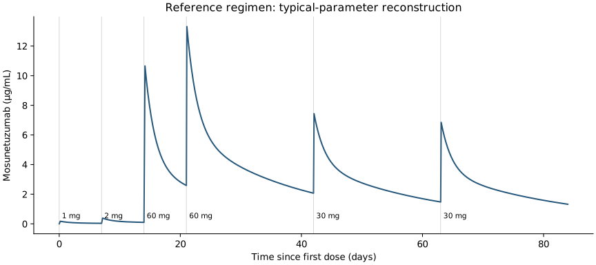
Figure 1. Concentration–time curve under the reference condition. Cycle 1 infusions were calculated as 4 hours and later infusions as 2 hours. Original calculation.
| Metric and unit | Published geometric mean | Recalculated typical value | Difference (%) |
|---|---|---|---|
| Cycle 1 AUC: µg·day/mL | 35.2 | 34.80 | -1.14 |
| Cycle 1 Cmax: µg/mL | 11.1 | 10.66 | -4.00 |
| Concentration at end of Cycle 1 interval: µg/mL | 2.6 | 2.59 | -0.42 |
| AUC 0–42: µg·day/mL | 126 | 125.08 | -0.73 |
| Cycle 4 AUC: µg·day/mL | 52.9 | 52.70 | -0.38 |
Reference values are based on the product information and Table S2 of the PopPK supplement. For the end-of-interval reference, 2.6 µg/mL, also given in Table 10 of the 2025 FDA label, was used.
AUC and end-of-interval concentration were close, but Cycle 1 Cmax differed by about −4.0%. Because Cmax also depends on infusion duration, the infusion was not treated as an instantaneous bolus.
Moreover, the published values are geometric means of model-predicted exposure in the patient population, a different statistic from the typical curve with reference covariates and η = 0 calculated here. This is not a reproduction using the same individual patient parameters and covariate distribution as the publication. This closeness is reference material confirming the consistency of the implementation; it does not mean independent external validation or reproduction of the patient population.
Result 2: regimen comparison within the same virtual patients
Each virtual patient's parameters were fixed, and both the reference and the modified regimens were given. The percentage change was calculated for each patient, and the median is shown in the table. This removes differences due to drawing different patients for each comparison group.
| Change | First Cmax | Concentration before first 60 mg | AUC 0–42 |
|---|---|---|---|
| First dose 1 → 0.5 mg | -50.0% | -11.0% | -0.4% |
| First dose 1 → 2 mg | +100.0% | +22.1% | +0.8% |
| Second dose 2 → 1 mg | +0.0% | -39.0% | -0.9% |
| Second dose 2 → 4 mg | +0.0% | +77.9% | +1.7% |
| Interval 7 → 3.5 days | +0.0% | +54.1% | +18.6% |
| Interval 7 → 14 days | +0.0% | -36.3% | -30.8% |
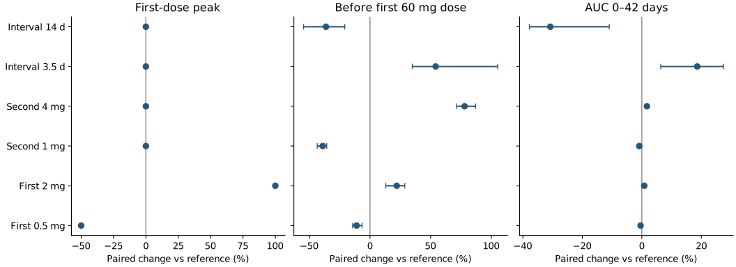
Figure 2. Points are medians of paired percentage changes, and horizontal lines are the 2.5th–97.5th percentiles across virtual patients, not 95% confidence intervals for estimates. The same 2,000 patients were used throughout. Original calculation.
The first and second doses mainly move near-term exposure
Under the same time-dependent CL, this PK model is linear in the dosing input. The first Cmax, measured before any other dose, is therefore proportional to the first dose: −50% at 0.5 mg and +100% at 2 mg. This exact proportionality is a property of the model, not a clinical proportional relationship for CRS.
Reducing the second dose to 1 mg changed the median concentration just before the first 60 mg dose by about −39%, and increasing it to 4 mg by about +78%. On the other hand, changing only the first or second dose changed the 42-day AUC by about −0.9% to +1.7%. In cumulative exposure, the later 60 mg doses contribute most.
Changing the interval also changes cumulative exposure
Shortening the interval to 3.5 days changed the concentration just before 60 mg by about +54%, and extending it to 14 days by about −36%. However, even though both are "just before 60 mg", the times compared differ: days 7, 14 and 28. The result combines residual drug, distribution and elimination, and time-dependent CL.
The 42-day AUC changed by about +19% with the shorter interval and about −31% with the longer interval. Unlike changes in the first or second dose, these are not small differences. Because the time at which the large doses enter and whether maintenance doses fall before day 42 also change, this is not interpreted as "the pure effect of the dosing interval on CL".
Result 3: which uncertainty was examined
Estimation uncertainty in the fixed effects
Each of the six fixed effects was replaced in turn with the lower and upper bounds of its published 95% CI. This is a one-at-a-time sensitivity analysis, not a probabilistic analysis that changes fixed effects simultaneously. Because the covariance matrix of the fixed-effect estimates is not available, the results are not called 95% confidence intervals for exposure.
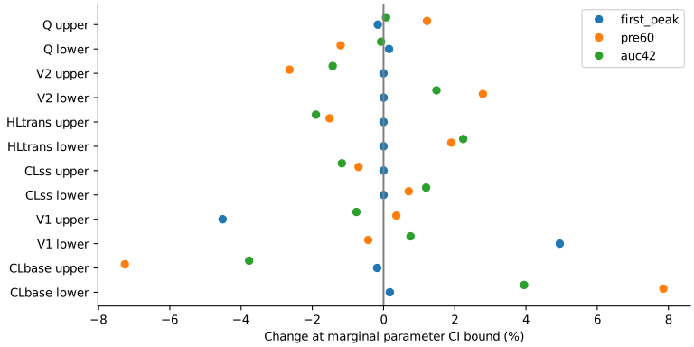
Figure 3. A local sensitivity analysis with the other parameters fixed. The conditions and values for each point are published as CSV. Original calculation.
The largest absolute changes were about 4.9% for the first Cmax, about 7.9% for the concentration before 60 mg and about 3.9% for the 42-day AUC. The changes in peak from changing the first dose, and in pre-dose concentration from changing the second dose or interval, are larger than this local fixed-effect sensitivity.
This is not a conclusion common to all metrics, however. The difference in 42-day AUC from changing only the first or second dose can be smaller than this parameter sensitivity. These CIs also cannot assess misspecification of the structural model or missing patient characteristics.
Between-subject variability
The absolute exposure for the reference regimen given to the virtual patients was as follows.
| Metric | Median | 2.5th–97.5th percentile |
|---|---|---|
| First Cmax (µg/mL) | 0.175 | 0.096–0.333 |
| Concentration before first 60 mg (µg/mL) | 0.101 | 0.032–0.191 |
| AUC 0–42 (µg·day/mL) | 123.830 | 55.519–193.473 |
Absolute exposure varies, but in the paired analysis the direction of the effects of changing the second dose or the interval was maintained. However, this population fixes the reference covariates and reflects only Ω; it does not reproduce the joint distribution of real patients' body weight, tumor burden, albumin, residual anti-CD20 and IIV. It has not been validated as the exposure distribution of a patient population.
Result 4: from PK to RO, and from RO to CRS
Binding competition with residual anti-CD20
The public RO model was implemented as follows, with all units in µg/mL.
\[ RO(t)=100\frac{C_M(t)}{C_M(t)+K_{D,M}+\frac{K_{D,M}}{K_{D,R}}C_R(t)+\frac{K_{D,M}}{K_{D,G}}C_G(t)} \]
Here M is mosunetuzumab, R is rituximab (RTX) and G is obinutuzumab (OBI), with \(K_{D,M}=10.2\), \(K_{D,R}=0.675\) and \(K_{D,G}=0.600\) µg/mL. RTX and OBI decline from their starting concentrations with half-lives of 24 and 28 days. The starting concentrations are not held constant over 42 days. RO equation and implementation in the PopPK supplement
The RO equation is an approximation of CD20 occupancy based on competitive binding. RO calculated from blood concentration is not equated with occupancy in tumor tissue or with a direct measurement of T-cell activation.
The published CRS equation uses the maximum RO over 42 days
For the step-up dosing group (Group B) of Study GO29781 in relapsed or refractory non-Hodgkin lymphoma, the published logistic equation for Grade ≥2 CRS by ASTCT criteria was used. This is not a model built only from patients with follicular lymphoma at the approved dose.
\[ \operatorname{logit}(p)=-2.64+0.0196\,RO_{max,0-42} \]
The RO input is a percentage from 0 to 100, not a proportion from 0 to 1. It is also the maximum RO over the first 42 days, not the maximum RO just after the first dose. Table S12 of the E–R supplement
The heading of Table S12 says Grade 2, but the Grade ≥2 definition in the text of the paper was followed. Standard errors of the coefficients are published as 0.279 for the intercept and 0.00804 for the slope, but their covariance is not, so no confidence interval was constructed for the output of the CRS equation.
This distinction matters. If a later 60 mg dose determines the maximum RO, changing the first dose may not move this metric much. That does not mean priming by the first dose or the dosing history is irrelevant to CRS. The regression has no state variable that mechanistically represents a modified dosing history.
Two assumptions about anti-CD20
First, PK was fixed and only competitive binding was changed. Next, the CLbase covariate effect of baseline anti-CD20 in the public PK model was also applied. In the published implementation, the covariate term is \([\log(ACD20)/\log(500)]^{-0.573}\), with baseline anti-CD20 in ng/mL.
For the binding condition with no residual drug, the reference value of 500 ng/mL was used in the covariate calculation. This is a reference condition in this analysis to avoid taking the log of 0, not a full reproduction of the original NONMEM imputation of missing values without patient data. The lower-bound handling in the code is not interpreted as a validated rule for patients below the limit of quantification in general.
| Baseline anti-CD20 | Max RO: binding only | CRS equation output: binding only | Max RO: CL also changed | CRS equation output: CL also changed |
|---|---|---|---|---|
| No residual drug | 56.63% | 17.80% | 56.63% | 17.80% |
| RTX 10 µg/mL | 12.60% | 8.37% | 12.81% | 8.40% |
| OBI 10 µg/mL | 10.71% | 8.09% | 10.89% | 8.12% |
| RTX 305 µg/mL | 0.53% | 6.73% | 0.54% | 6.73% |
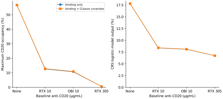
Figure 4. A sensitivity analysis for the reference regimen in a typical patient. The lines connecting points are for ease of comparison, not continuous dose–response curves between drugs. The CRS equation output is not an individual risk prediction. Original calculation.
Under these conditions, the difference due to competitive binding in the RO equation was larger than the difference due to applying the CLbase covariate. There is, however, no basis for mixing the four concentration conditions into a population in equal proportions, or for taking the table in this article as the incidence in real patients.
In particular, even as RO approaches 0, the regression output is about 6.7%. This is a property of the intercept, not a number that independently demonstrates residual pharmacological risk. The probability a simple equation produces includes the effects of the original analysis population and conditions.
What can and cannot be said
| Subject of judgment | What this analysis supports | What it does not support |
|---|---|---|
| PK implementation | Independently implemented the structural equations and dosing events and confirmed numerical consistency | External validation with new patient data |
| Dose comparison | Exposure changes within the same model and the same patient parameters | A guarantee that the model has the same clinical accuracy after the change |
| Uncertainty | Local fixed-effect sensitivity and individual differences based on Ω | A full predictive distribution integrating fixed effects, covariates and model structure |
| RO–CRS | How much results depend on assumptions about residual drug and the regression | Population CRS incidence for a modified regimen, individual risk, the optimal regimen |
Patient-level PK observations, the joint distribution of covariates and residual anti-CD20 concentrations, and data linking CRS timing with dosing history were not available from the public materials used here. There are also no data to check whether the original RO–CRS relationship transports to hypothetical 3.5-day or 14-day intervals.
This evidence alone does not allow the conclusion that "the PK model has been qualified" on the basis of closeness to published values. What this analysis achieved is verifying the computational implementation of the public PK model and comparing regimen exposure within that model. The translation to RO–CRS can be explored as a sensitivity analysis but cannot be validated as a prediction of incidence in a patient population.
Code and results for rerunning
The analysis was run with Python 3.12. The random numbers for the virtual patients, the libraries used and the numerical integration settings are saved in the run record.
- Analysis code: run_analysis.py
- Dependencies: requirements.txt
- How to run and assumptions: README
- Comparison with published values (CSV)
- Paired regimen comparison (CSV)
- Reference exposure in the virtual population (CSV)
- Fixed-effect sensitivity (CSV)
- Anti-CD20 sensitivity (CSV)
python -m pip install -r requirements.txt
python run_analysis.py
The figures and tables are this article's own simulation results using published data as input, not measured patient data.
References and sources
- Bender B, et al. Population pharmacokinetics and CD20 binding dynamics for mosunetuzumab in relapsed/refractory B-cell non-Hodgkin lymphoma. Clinical and Translational Science. 2024;17:e13825. DOI: 10.1111/cts.13825. Supplement.
- Li CC, et al. A Novel Step-Up Dosage Regimen for Enhancing the Benefit-to-Risk Ratio of Mosunetuzumab in Relapsed or Refractory Follicular Lymphoma. Clinical Pharmacology & Therapeutics. 2025;117:465–474 (published online 2024). DOI: 10.1002/cpt.3445. Supplement.
- LUNSUMIO (mosunetuzumab-axgb), intravenous prescribing information. DailyMed; FDA 2025 label.
Sources checked: 2 October 2026. Analysis and writing: Daiki Kumakura.
Cite this article
Kumakura, D. (2026). Reimplementing a published mosunetuzumab population PK model: step-up dosing exposure and the limits of extrapolating to receptor occupancy and CRS. daikikumakura.github.io. https://daikikumakura.github.io/writing/mosunetuzumab-public-pk-en.html