Does a model that predicts well understand the mechanism? Separating prediction from mechanistic inference
On this page
- Abstract
- Introduction
- Scope and sources
- Prediction and mechanistic inference target different quantities
- A trade-off between model identification and regression estimation
- Virtual Cell metrics and baselines
- Conditions for identifying intervention effects
- Identifiability of mechanistic parameters
- A numerical example of non-identifiability and prediction
- Discussion
- Conclusion
- Data and code availability
- References
Abstract
Predictive accuracy, prediction under intervention and mechanism identification target different quantities. Selected work on model selection, perturbation prediction, identifiability and public model-evaluation frameworks is compared with a synthetic turnover-model example. Coefficients fitting similarly gave close predictions for slowly changing exposure but diverged sharply in unobserved early hours. Predictive stability and mechanistic identification therefore require separate assessment for the intended question and measurement design.
Literature and public materials checked on October 6, 2026.
Introduction
A model predicts unseen data extremely well. Can the relationships it represents internally be interpreted as disease or pharmacological mechanisms?
Conversely, if a model is “mechanistic,” built from ODEs or reaction networks, can its parameters and structure be trusted as biological mechanisms?
Both claims require additional evidence. Prediction and mechanistic inference overlap, but they are not the same optimization problem. Prediction claims need predictive tests; mechanism claims need tests of mechanisms. A model claiming both should face both.
Scope and sources
The comparison covers statistical model selection, causal inference, single-cell perturbation prediction, dynamic-model identifiability and public evaluation frameworks. It uses selected literature and a synthetic example, rather than an exhaustive review or validation of an actual drug mechanism.
Prediction and mechanistic inference target different quantities
A simplified prediction objective selects a function minimizing expected loss on unseen data:
\[ f^{*}=\arg\min_{f}\ \mathbb{E}\left[L\bigl(Y,f(X)\bigr)\right] \]
Mechanistic questions instead include whether inhibiting a protein changes downstream signaling, whether receptor occupancy mediates an exposure–effect relationship, or whether a biomarker–prognosis association represents an actionable pathway.
These are not one type of question. I distinguish at least three layers:
- Prediction under observation: predict another observation under comparable conditions, targeting \(P(Y\mid X)\).
- Prediction under intervention: predict Y when A changes, targeting \(\mathbb{E}[Y\mid do(A=a)]\), or its difference between \(a_1\) and \(a_0\).
- Mechanistic claims: specify the pathways and mediators producing an effect. Whether receptor occupancy mediates an effect concerns mediation, rather than the total intervention effect.
Accurate observational prediction does not establish the second or third layer. Accurate intervention prediction does not by itself establish the pathway in the third.
Hernán and colleagues distinguish description, prediction and counterfactual prediction, including causal inference (1). In clinical prediction, van Geloven and colleagues explain why predicting risk without treatment versus under current practice changes both the estimand and data handling (2). Counterfactual prediction is also not exclusively for causal inference (3). The starting point here is likewise to write down the estimand first.
“Identification” has two meanings in this article. Causal identification asks whether an intervention effect is uniquely determined from an observational distribution; parameter identifiability asks whether model parameters are uniquely determined by data. The causal-identification section concerns the former; parameter identifiability and the numerical example concern the latter.
A trade-off between model identification and regression estimation
Yuhong Yang's 2005 paper offers an interesting starting point (4). It asks whether one regression-model selection criterion can combine BIC-type consistency, selecting the true finite-dimensional candidate model with probability approaching one, and an AIC-type minimax rate for estimating the regression function. The answer is negative: a consistent model-selection criterion cannot achieve the optimal worst-case minimax convergence rate for regression estimation. Bayesian model averaging cannot be minimax-rate optimal in that sense either.
This is not a general theorem that prediction models cannot support causal inference. It concerns particular regression-selection settings and a mathematical trade-off between model identification and regression-function estimation. It is neither a theorem about causal identification nor a claim that every dataset incurs a loss.
It nevertheless warns against assuming that one “best model” is automatically best for different scientific purposes. Changing what counts as correct can change the optimal selection procedure.
Galit Shmueli systematically argued for distinguishing explanation from prediction in 2010 (5). Explanatory models emphasize the meaning of variables and structure; predictive models are assessed by generalization to unseen data. Confusing the two invites opposite leaps: “it predicts well, so this variable is causal,” or “the mechanism sounds plausible, so it must predict unseen patients well.”
Virtual Cell metrics and baselines
Single-cell perturbation prediction illustrates these distinctions. A separate article examines its evaluation metrics (6); here I retain the points needed for this argument.
Perturb-seq already measures outcomes of genetic interventions. The issue is therefore not simply observation versus intervention. It is generalization to unseen perturbations or cellular backgrounds, and whether predicting intervention outcomes recovers the underlying pathway or network: the distinction between layers two and three.
In 2025, Ahlmann-Eltze and colleagues compared five foundation models and two deep-learning models against deliberately simple baselines. None exceeded the baselines for transcriptional changes following single or double perturbations (7). That does not make deep learning useless for biology. It means model complexity or expressive capacity alone does not establish value for a specified prediction task.
Across ten datasets, Systema showed that shared systematic differences between perturbed and control cells can inflate common metrics regardless of perturbation identity (8). A high score need not establish perturbation-specific response prediction.
On October 1, 2026, Miller and colleagues added an important argument in the other direction (9). Across 14 datasets and 18 metrics, positive-control predictions and uninformative baselines showed that some common metrics, including MSE and Pearson correlation of control-relative changes, had low sensitivity to genuinely informative predictions. More sensitive, “well-calibrated” metrics detected deep-learning improvements in some settings. Calibration here means distinguishing informative from uninformative predictions, rather than calibrating predicted probabilities.
Taken together, these papers resist a simple verdict. Complex models can lose to simple references, while insensitive metrics can hide real predictive information. Predicting intervention effects still differs from recovering the correct mechanism.
Evaluation is an experiment comprising the split, baseline, loss and metric, not just the model. The 2026 Virtual Cell Challenge's zero-shot prediction into cellular backgrounds without perturbation data, and ranking by six aggregated metrics, fit this concern (10). Final results were unavailable when sources were checked; this article does not predict them.
Conditions for identifying intervention effects
Identification in this section is causal. Consider
\[ U\rightarrow X,\quad U\rightarrow Y,\quad X\rightarrow M\rightarrow Y,\quad X\rightarrow Z \]
\(U\) is an unmeasured common cause, \(M\) a mediator and \(Z\) a downstream proxy that does not affect Y. Suppose X and M move almost perfectly together in the observed data.
Either \(Y=f(X)\) or \(Y=g(Z)\) might predict accurately, yet intervention questions differ:
- Manipulating Z does not change Y; the accuracy of g(Z) establishes no effect of Z.
- The effect of intervening on X differs from \(P(Y\mid X)\), which includes association through U. Obtaining \(P(Y\mid do(X))\) needs additional conditions such as adjustment for U, interventional data or external structural knowledge.
- Inhibiting M alone is effectively extrapolation if almost no observations vary M independently of X: positivity is nearly absent.
In a simple unconfounded \(X\rightarrow M\rightarrow Y\) system whose other relationships remain unchanged under intervention, \(P(Y\mid do(X))=P(Y\mid X)\). Prediction and intervention can agree. Confounding, selection, proxies and extrapolation to absent variation can make them diverge; establishing their absence in real data is often difficult.
Large SHAP values, attention weights or feature importance cannot alone establish a mechanism. They primarily describe how an input is used within the predictor, rather than intervention effects. The official SHAP documentation itself devotes a section to caution about extracting causal insights from predictive-model interpretation (11).
Identifiability of mechanistic parameters
There is an opposite trap. Identification here and in the next section concerns parameters.
Suppose a turnover model represents drug-induced removal of a response R, such as target abundance or a biomarker:
\[ \frac{dR}{dt}=k_{\mathrm{in}}-k_{\mathrm{out}}R-k_{\mathrm{drug}}C(t)R, \qquad R(0)=R_0=\frac{k_{\mathrm{in}}}{k_{\mathrm{out}}} \]
This is the stimulated-loss form of Jusko and colleagues' indirect-response models with a linear drug effect. Defining \(S=k_{\mathrm{drug}}/k_{\mathrm{out}}\) gives \(\dfrac{dR}{dt}=k_{\mathrm{in}}-k_{\mathrm{out}}\bigl(1+S\,C(t)\bigr)R\); S is the conventional slope parameter for that form (12, 13). Its terms have mechanistic interpretations: production, turnover, exposure and stimulation of removal.
Observing only R(t), however, need not identify \(k_{\mathrm{in}}\), \(k_{\mathrm{out}}\) and \(k_{\mathrm{drug}}\) precisely. At least two problems differ.
Structural identifiability asks whether infinitely accurate observations uniquely determine parameters. With dose known but C(t) unmeasured, one-compartment PK gives \(C(t)=\mathrm{Dose}/V\cdot e^{-k_et}\). The response contains only the ratio \(k_{\mathrm{drug}}/V\). Response data alone cannot separate volume V from drug-effect strength.
Practical identifiability asks whether actual observation times, counts and errors constrain parameters narrowly enough. Structurally identifiable models can still yield nearly identical responses from different parameter combinations. “Sloppy” sensitivities, where many combinations weakly affect outputs, are common in systems biology (14). Profile likelihood can diagnose structural and practical non-identifiability (15), and related methods obtain confidence intervals for predictions rather than parameters (16).
The structure itself can also be wrong. A well-fitted ODE does not prove that nature follows that ODE. Mechanistic models need checks on structural and practical identifiability, misspecification, and validation with external data or intervention experiments.
A numerical example of non-identifiability and prediction
Methods
I examined the turnover model with synthetic data. True values were \(k_{\mathrm{out}}=2\)/day and \(S=0.075\) L/mg, or \(k_{\mathrm{drug}}=0.15\) L/mg/day. A single 100-mg IV dose followed one-compartment PK with V=5 L, \(k_e=0.1\)/day, half-life about 6.9 days and R0=100. R was observed on days 1, 2, 4, 7, 14, 21 and 28, with log-scale measurement SD 0.10 and seed 20261024. R0, C(t) and error SD were treated as known when calculating the likelihood of kout and S.
Known C(t) makes this model structurally identifiable. The example concerns practical non-identifiability caused by placing the first sample one day after dosing.
Likelihood was evaluated on a two-dimensional grid: 81 logarithmically spaced kout values from 0.1 to 1,000/day and 121 S values from 0.03 to 0.15. Reported intervals are minima and maxima among 1,619 points satisfying \(2\Delta\mathrm{NLL}\le3.84\), a grid approximation to 95% profile-likelihood intervals for each quantity.
Results
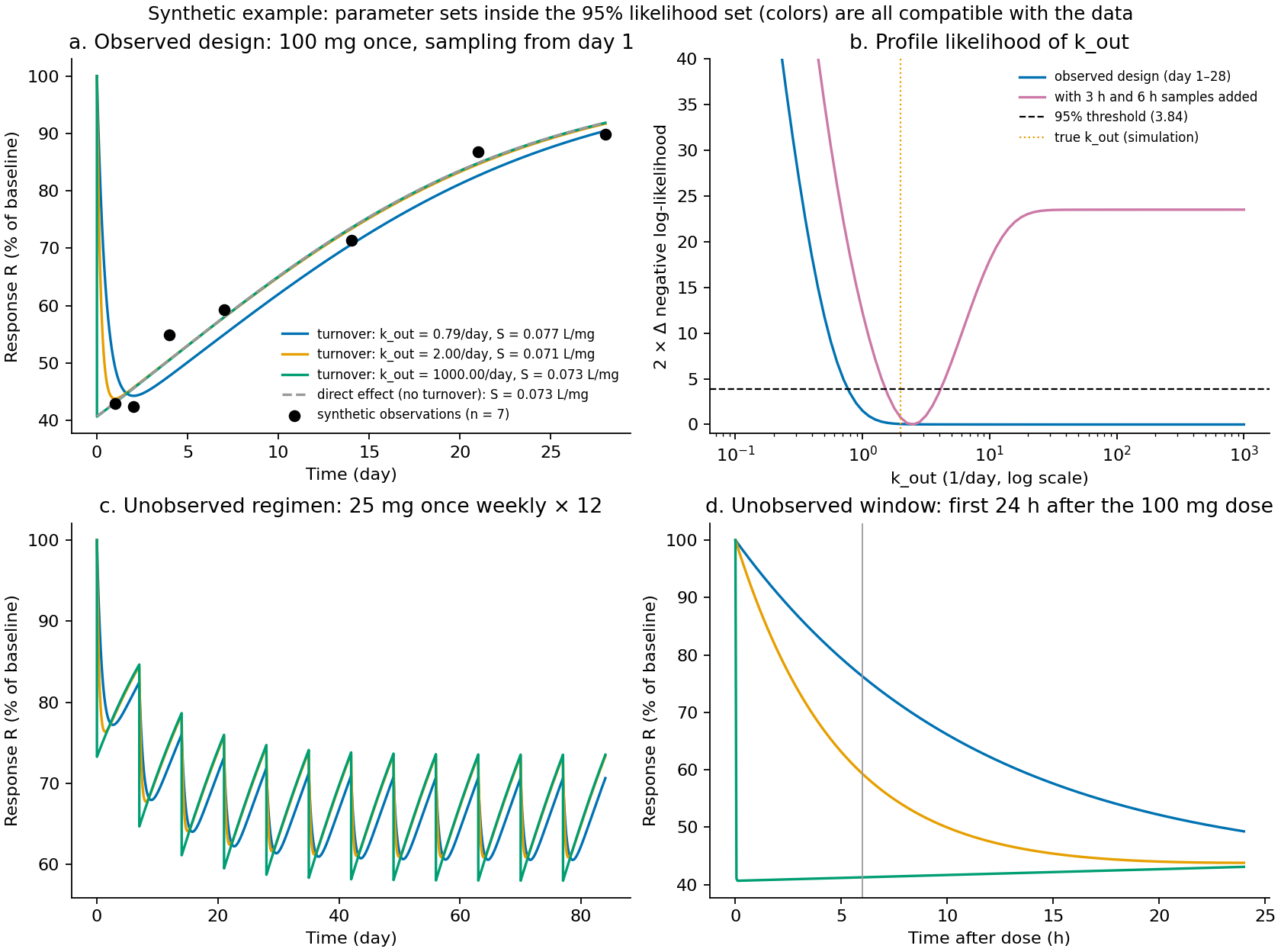
Figure 1. Synthetic data, not real observations. (a) Observations and fits for three parameter pairs in the likelihood region used to obtain the 95% profile intervals; both kout and S differ slightly. Gray dashes show the instantaneous direct-effect model \(R=R_0/(1+S\,C)\). (b) kout profile likelihood: blue is the original design, purple adds samples at three and six hours; dashed threshold is 3.84, the one-degree-of-freedom 95% chi-square point. (c) Unobserved dosing of 25 mg weekly for 12 doses. (d) The first 24 h after 100 mg, with a vertical line at six hours.
Figure 1 and Table 1 summarize the results. Outputs are results/summary.json, results/likelihood_set.csv and results/kout_profile.csv.
Table 1. Parameter and prediction intervals
| Quantity | 95% interval, grid approximation | Range holding S=0.073 and varying only kout |
|---|---|---|
| kout (/day) | Lower bound about 0.77; no upper bound | — |
| S (L/mg) | 0.059–0.086; true 0.075 | — |
| R on day 84 with 25 mg weekly | 69.2–77.1 | 71.7–73.5 |
| Minimum R during 25 mg weekly | 54.0–65.2 | 58.0–61.9 |
| R six hours after 100 mg | 37.3–77.3 | 41.2–77.3 |
First, kout has only a lower bound. Likelihood improves slightly as kout increases, and no interior minimum was obtained on the explored grid: the negative log likelihood was smallest at its boundary of 1,000/day. Even noiseless data at the true values give only 0.017 for \(2\Delta\mathrm{NLL}\) at kout=1,000. The absent upper bound reflects the observation design rather than just this random realization.
Second, the observations cannot distinguish a delayed response from an effectively instantaneous response. Earlier measurements are needed to resolve the delay. The best negative log likelihood of the direct-effect model, 0.72033, matches that of the turnover model, 0.72034. The direct-effect model is its \(k_{\mathrm{out}}\to\infty\) limit. When concentration changes much more slowly than turnover, \(R\approx R_0/(1+S\,C)\), so the data primarily identify S. Such time-scale separation in indirect-response models has long been recognized (12, 13).
Third, whether non-identifiability matters depends on the question. Uncertainty for 25 mg weekly in Figure 1c mainly comes from S. At fixed S, varying kout from about 0.8 to 1,000/day within the likelihood set changes day-84 R by only about two units and the minimum by about four. In the unobserved first hours, the same variation changes six-hour R from about 41 to 77. Weekly dosing still has concentration changes slower than turnover except immediately after each dose, permitting a quasi-steady approximation. The residual four-unit minimum difference comes from those transients. Short-half-life drugs or regimens with concentration changes over hours can violate that condition.
Fourth, additional early observations narrowed the interval in this example. The fitted lower bound near 0.77/day suggests a response time scale at most roughly a day. True target half-life without drug, \(\ln2/k_{\mathrm{out}}\), is about eight hours, shortened to about three hours immediately after dosing. Adding three- and six-hour observations narrows the 95% kout interval to about 1.5–4.1/day in this random realization (purple in Figure 1b). A specified question indicates which times need measurement.
Failure to estimate kout therefore does not automatically make the model useless. Comparisons of slowly changing exposure regimens can remain answerable within S uncertainty. The necessary check is whether the data determine the parameter combinations on which the question depends.
This calculation assumes the structure is correct and remains invariant with regimen changes. That is analogous to the causal-identification assumptions and is stipulated in the simulation; real applications require intervention data to test it. The example illustrates one mechanism and establishes nothing about a particular actual drug or target.
Numerical implementation checks and limits
The ODE is linear in R. At 0.002-day steps, each interval uses the midpoint loss rate and an analytic interval solution, an exponential-integration method. The independent check compares weekly 25-mg predictions against Radau at tolerance \(10^{-10}\): differences were below \(10^{-5}\) at kout=2/day and about 0.001 R units at the grid boundary kout=1,000/day.
Measurement SD, R0 and concentration profiles are known. Interindividual variability, PK uncertainty and misspecification are omitted. Grid-based interval endpoints depend on resolution, including S steps of 0.001. The kout lower bound uses linear interpolation on the log scale between grid points. A chi-square-based 95% threshold remains approximate when parameters move toward a boundary.
Discussion
For predicting tumor size at the next measurement, predictive performance takes priority. If carrying the last observation forward beats a complex tumor-growth model, that purpose can favor the simpler predictor.
Asking why efficacy persists at a longer dosing interval is different. Without distinguishing the roles of AUC, Cmax, Cmin, target turnover and receptor occupancy, extrapolation to an unobserved regimen can fail. Prediction within an existing dose range requires different assumptions from
\[ \text{unobserved dose}\rightarrow\text{unobserved exposure profile}\rightarrow\text{response} \]
In the numerical example, predictions agreed where exposure changed more slowly than turnover and diverged immediately after dosing. A mechanistic model's value comes from specifying what should remain invariant and what should change under a different intervention, beyond goodness of fit alone.
Regulatory frameworks also start from questions and decision consequences rather than model labels. ICH M15, adopted at Step 4 on January 29, 2026, specifies the question of interest and context of use, assesses model risk from its influence on the decision and the consequences of error, then determines required credibility evidence. Its examples include PopPK, PBPK, exposure–response, QSP, disease progression and AI/ML (17). The FDA issued final M15 guidance in June 2026 (18).
For AI, a January 2025 FDA draft describes a seven-step, risk-based credibility framework by context of use; it remained a draft when checked (19). FDA and EMA jointly published ten good-AI principles in January 2026 covering the development lifecycle (20). Those high-level principles include early research without specifying a detailed assessment procedure. The FDA draft, by contrast, excludes discovery-stage uses. Extending its credibility framework to a research application such as Virtual Cell is an analogy made here.
In these terms, the same model requires different evidence when its question and role in a decision differ. Prediction under observed conditions, extrapolation to unobserved interventions and mechanistic claims have different risks and validation requirements.
Predictive performance and mechanism evidence
Prediction performance is defined for populations and conditions. Equal discrimination can conceal different calibration; low error under known conditions can coexist with failed intervention extrapolation.
Mechanistic evidence includes identifiability, prediction in other conditions with fixed coefficients and correspondence to measured mediators. These differ from fit, so
\[ \text{model quality}\neq\text{one scalar value} \]
The example likewise shows why one goodness-of-fit value cannot simultaneously establish predictive stability and mechanism identification.
Conclusion
Yang's result concerns a bounded statistical problem, but proves that model identification and regression estimation can conflict mathematically. In single-cell perturbation prediction, baselines and metrics also change what “successful prediction” establishes.
Here the delayed-response and instantaneous-response models fit similarly. Coefficients in the likelihood region used to obtain the 95% profile intervals produce close weekly-regimen predictions but diverge sharply immediately after dosing. Fit alone does not identify the short-term response or its mechanism.
Data and code availability
Extract the reproduction ZIP and run the following from its directory with Python 3.11 or later. Tested NumPy, SciPy and Matplotlib versions are pinned in requirements.txt. Runtime is about two to four minutes, depending on the environment.
python -m pip install -r requirements.txt
python identifiability_demo.py
The calculation code generates results/likelihood_set.csv, results/kout_profile.csv, results/summary.json and Figure 1.
References
- Hernán MA, Hsu J, Healy B. A Second Chance to Get Causal Inference Right: A Classification of Data Science Tasks. CHANCE. 2019;32(1):42–49. doi:10.1080/09332480.2019.1579578.
- van Geloven N, Swanson SA, Ramspek CL, Luijken K, van Diepen M, Morris TP, et al. Prediction meets causal inference: the role of treatment in clinical prediction models. European Journal of Epidemiology. 2020;35(7):619–630. doi:10.1007/s10654-020-00636-1.
- Dickerman BA, Hernán MA. Counterfactual prediction is not only for causal inference. European Journal of Epidemiology. 2020;35(7):615–617. doi:10.1007/s10654-020-00659-8.
- Yang Y. Can the strengths of AIC and BIC be shared? A conflict between model identification and regression estimation. Biometrika. 2005;92(4):937–950. doi:10.1093/biomet/92.4.937.
- Shmueli G. To Explain or to Predict?. Statistical Science. 2010;25(3):289–310. doi:10.1214/10-STS330.
- Kumakura D. What did the Virtual Cell predict? Target genes and evaluation shortcuts [Internet; technical note]. 2026 Oct 11. English article.
- Ahlmann-Eltze C, Huber W, Anders S. Deep-learning-based gene perturbation effect prediction does not yet outperform simple linear baselines. Nature Methods. 2025;22(8):1657–1661. doi:10.1038/s41592-025-02772-6.
- Viñas Torné R, Wiatrak M, Piran Z, Fan S, Jiang L, Teichmann SA, et al. Systema: a framework for evaluating genetic perturbation response prediction beyond systematic variation. Nature Biotechnology. 2026;44(6):1050–1059. doi:10.1038/s41587-025-02777-8.
- Miller HE, Mejia GM, Leblanc FJA, Swain B, Wang B, de Lima Camillo LP. Deep learning perturbation models can outperform baselines on calibrated metrics. Nature Biotechnology. 2026 [published online 2026 Oct 1]. doi:10.1038/s41587-026-03307-w.
- Arc Institute. The 2026 Virtual Cell Challenge: predicting perturbation responses in cell contexts a model has never seen [Internet]. 2026 Aug 20 [cited 2026 Oct 6]. Announcement. The published schedule lists final test-set release on Oct 22 and final submissions on Nov 5.
- SHAP documentation. Be careful when interpreting predictive models in search of causal insights [Internet; cited 2026 Oct 6]. Official documentation.
- Dayneka NL, Garg V, Jusko WJ. Comparison of four basic models of indirect pharmacodynamic responses. Journal of Pharmacokinetics and Biopharmaceutics. 1993;21(4):457–478. doi:10.1007/BF01061691.
- Sharma A, Jusko WJ. Characteristics of indirect pharmacodynamic models and applications to clinical drug responses. British Journal of Clinical Pharmacology. 1998;45(3):229–239. doi:10.1046/j.1365-2125.1998.00676.x.
- Gutenkunst RN, Waterfall JJ, Casey FP, Brown KS, Myers CR, Sethna JP. Universally Sloppy Parameter Sensitivities in Systems Biology Models. PLoS Computational Biology. 2007;3(10):e189. doi:10.1371/journal.pcbi.0030189.
- Raue A, Kreutz C, Maiwald T, Bachmann J, Schilling M, Klingmüller U, et al. Structural and practical identifiability analysis of partially observed dynamical models by exploiting the profile likelihood. Bioinformatics. 2009;25(15):1923–1929. doi:10.1093/bioinformatics/btp358.
- Kreutz C, Raue A, Timmer J. Likelihood based observability analysis and confidence intervals for predictions of dynamic models. BMC Systems Biology. 2012;6(1):120. doi:10.1186/1752-0509-6-120.
- International Council for Harmonisation. General principles for model-informed drug development: M15 [Guideline; Step 4]. 2026 Jan 29. Final guideline.
- US Food and Drug Administration. M15 General Principles for Model-Informed Drug Development [Internet; final guidance]. 2026 Jun. Official guidance.
- US Food and Drug Administration. Considerations for the Use of Artificial Intelligence To Support Regulatory Decision-Making for Drug and Biological Products [Internet; draft guidance]. 2025 Jan. Official draft guidance.
- European Medicines Agency; US Food and Drug Administration. Guiding principles of good AI practice in drug development [Internet]. 2026 Jan. Joint principles. EMA announcement.