When a model fails to beat the baseline, what should we measure next?
On this page
- Abstract
- Introduction
- Cell counts and distinguishable conditions
- Information depends on the observation conditions
- What perturbation-prediction papers compare
- Add information beyond cell counts
- What an additional experiment is meant to achieve
- Discussion
- Conclusion
- Data and code availability
- References
Abstract
Failure to detect improvements in perturbation prediction can reflect insufficient data information, incomplete use of information by a model, or insensitive evaluation metrics. Selected literature is compared with information-matrix calculations for exponential decay and expected whole-gene MSE. Replication under one condition can sharpen its mean without separating non-identifiable parameters, while adding unchanged genes dilutes improvements in aggregate MSE. Appropriate observations and evaluations depend on the prediction target and experimental objective.
Literature checked on October 9, 2026. This article distinguishes peer-reviewed papers, preprints and developer reports. Its figures and numerical tables are mathematical examples, not reanalyses of measured perturbation data.
Introduction
When a new model cannot beat a predictor that returns the mean, two questions need separate consideration: Do the data contain the difference we want to predict? Does the evaluation detect that difference?
These are separate problems. Some quantities cannot be estimated from uninformative observations. Yet a model may also fail to use information that is present, or an evaluation may miss a real improvement. A failure to beat the baseline does not distinguish these possibilities.
In a May 2025 blog post (1), Eric Kernfeld argued that gene regulatory network inference should consider data informativeness and the additional observations needed before focusing on model ingenuity. That is the starting point here, too. It is a view about research strategy, not an impossibility proof for all perturbation prediction.
Cell counts and distinguishable conditions
Single-cell datasets can contain large numbers of cells. More cells from one condition, however, do not supply the same information as measurements at another time, under another perturbation or in another background.
More cells characterize a condition's mean and distribution more precisely. A single time point does not directly reveal what happened earlier. A single cell line does not test transfer to another line. Even with many cells, few independent experimental batches or donors leave uncertainty that cell counts alone cannot remove.
Ten thousand cells from one culture, for example, should not automatically count as ten thousand independent biological replicates. Variation among cells under the same condition needs to be distinguished from variation across cultures, donors and experimental days. Generalization across the latter requires independent replication.
This does not make additional cells useless. The question is which uncertainty an additional observation reduces.
Information depends on the observation conditions
Consider a decaying response:
\[ y(t)=A\exp(-kt)+\varepsilon,\qquad \varepsilon\sim N(0,\sigma^2). \]
Assume independent measurement errors with known, constant variance. If amplitude \(A\) is known, the Fisher information about decay rate \(k\) is
\[ I_k=\frac{A^2}{\sigma^2}\sum_r t_r^2\exp(-2kt_r) \]
Repeated measurements at time zero supply no information about \(k\). Information per observation is maximal at \(t=1/k\), but only for this model, with known amplitude and independent constant-variance errors. More unknown parameters can change the best observation times.
If amplitude is also unknown, repeated measurements at a single positive time \(t_0\) identify only \(A\exp(-kt_0)\). Infinitely many amplitude–rate pairs give that value. More replicates sharpen the mean at that time without separating the two parameters.
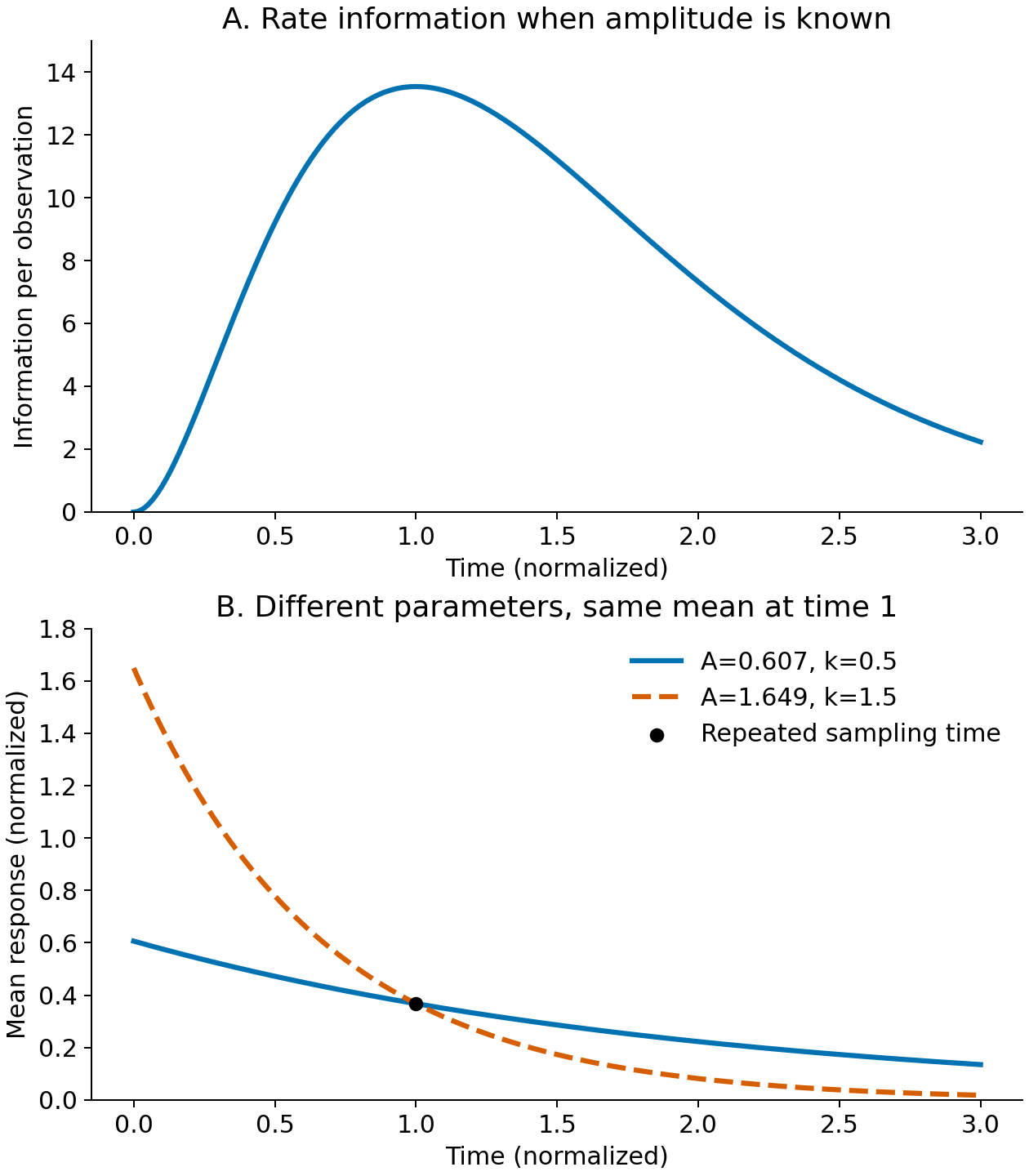
Figure 1. Observation times and identifiability. An illustrative calculation in normalized units. The upper panel uses \(A=k=1,\sigma=0.1\). The two curves below have identical means at time one. No exponential decay was fitted to actual cellular responses.
Even with ten measurements in every design, their allocation changes the rank of the information matrix for amplitude and rate. Table 1 is a local calculation for \((\log A,\log k)\).
Table 1 Observation-time allocation and local information
| Allocation of ten measurements | Information matrix rank | Local information about log k accounting for uncertain amplitude |
|---|---|---|
| All at time zero | 1 | 0 |
| All at time one | 1 | 0 |
| Five at time zero and five at time one | 2 | 59.60 |
Output: results/designs.csv. Conditional information with amplitude fixed must be distinguished from information with amplitude unknown. Two time points permit local separation in this example, but sufficiently precise estimation from real data requires a separate check.
For practical models, profile likelihood fixes each parameter in turn and re-estimates the others. Raue et al. (2) address both structural non-identifiability and practical limitations from finite data. A flat likelihood alone is not a general impossibility result: model symmetries, observation design, error assumptions and the search range also matter.
What perturbation-prediction papers compare
Reducing recent discussions to whether deep learning wins or loses hides the differences that matter. Baselines, predicted outputs and definitions of an unseen condition vary.
Table 2 Comparison targets in perturbation-prediction studies
| Primary source | Release and status | Point examined here |
|---|---|---|
| Ahlmann-Eltze et al. (3) | August 2025; peer-reviewed | Strong simple linear baselines in the examined settings, rather than a conclusion about all future models |
| Systema (4) | Online August 2025; peer-reviewed | Separate evaluation of shared perturbation variation and target-specific responses |
| Wei et al. (5) | Online December 2025; peer-reviewed | Comparison of 27 methods, 29 datasets and six metrics; unseen perturbations and unseen backgrounds require separate interpretation |
| Miller et al. (6) | October 1, 2026; peer-reviewed | Fourteen datasets and 18 metrics; positive controls test metric sensitivity and detect deep-model improvements in some settings |
| AmbiModBench (7) | September 26, 2026; preprint | Training-mean comparisons, gene-coordinate permutation and representation-space coverage probe what a score measures |
Miller and colleagues use technical duplicates made by splitting cells from the same perturbation, and interpolated duplicates that move weak responses toward the mean, to examine how well metrics distinguish positive and negative controls. A technical duplicate is an estimate from finite cells: for a weak signal it can vary more than a mean baseline. It is neither an oracle that knows the true conditional mean nor a guarantee of reproducibility across independent biological experiments.
The paper also compares linear and additive baselines. Models outperforming additivity were reported for combination prediction in Wessels23, whereas additivity was strong in Norman19. Training coverage, response strength, dataset composition and model generation differ, so a single cause cannot be assigned to the difference. Neither universal failure nor universal success follows. This study also did not test generalization to unseen cellular backgrounds.
Calibration here means checking evaluation metric sensitivity, rather than calibrating predicted probabilities. A positive control constructed from measured test responses is not a predictor deployable on an unseen condition. Using test-derived controls to assess a scoring system must be separated from feeding that information back into training or model selection.
A simple expectation illustrates how evaluation can dilute improvements. Suppose only ten of \(G\) evaluated genes change by one unit, with independent observation errors of variance one for every gene. A predictor of no change has expected MSE \(1+10/G\), whereas an oracle knowing the true conditional mean has expected MSE one.
Table 3 Evaluated gene counts and expected MSE
| Evaluated genes | Expected MSE predicting no change | Expected MSE knowing the true mean | Difference |
|---|---|---|---|
| 100 | 1.100 | 1.000 | 0.100 |
| 1,000 | 1.010 | 1.000 | 0.010 |
| 10,000 | 1.001 | 1.000 | 0.001 |
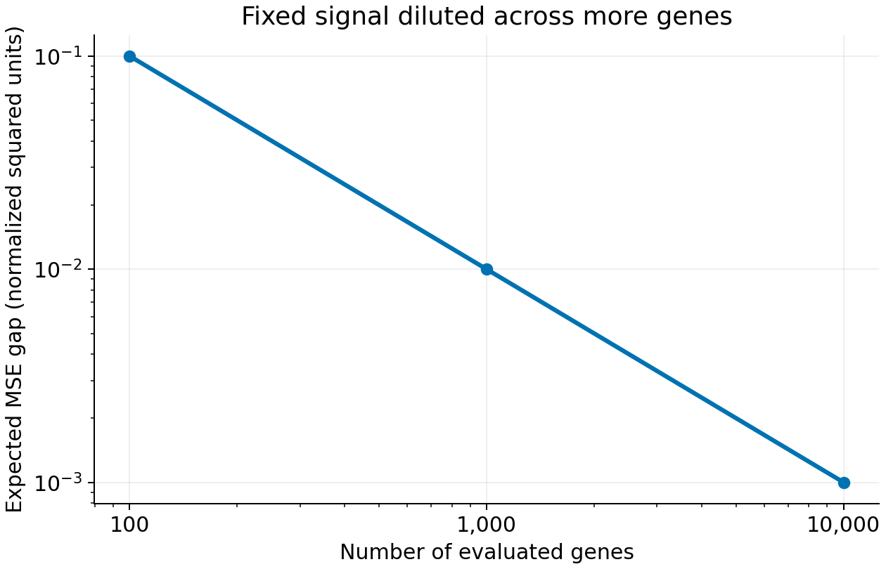
Figure 2. Dilution of a fixed signal. Both axes are logarithmic. Output: results/metrics.csv. The ranking never reverses in this example: the oracle is always better. A small difference is also not the same as a statistically undetectable difference. Sufficient independent replication may detect a small effect.
This figure does not reproduce the Miller evaluation; it illustrates dilution within an aggregate metric. Selecting only changed genes in real data can introduce new evaluation bias unless the selection procedure and controls are specified.
Add information beyond cell counts
Another observation layer or background information can distinguish relationships that RNA alone does not resolve. LINGER (8) infers regulatory networks using RNA, chromatin and external information. Benchmark improvements do not establish that every inferred edge is causal, but they offer a concrete example of expanding inputs.
Reports in 2026 also examine observation quality and background coverage. A preprint by Wang et al. (9) checks perturbation efficacy and separation of shared from specific responses. Its classifications depend on study-specific definitions; they should not become a universal claim that some fixed proportion of public datasets is unusable.
The peer-reviewed State paper (10) addresses collections of cells and transfer across backgrounds. PIE, released October 5 (11), is a preprint predicting population-level responses from prior biological knowledge and perturbation data. Its developer explanation (12) also shows lower accuracy when both cellular context and perturbation are unseen. This is an author report, rather than an independent replication.
When improvements change input knowledge and output definitions, as in PIE, calling the result simply a victory for larger models is misleading. Comparisons need to check the origin and availability date of external knowledge, pretraining targets and overlap with evaluation conditions. Using external knowledge is not inherently improper; its availability in the intended application is what matters.
Arc's 2026 data-generation report (13) describes harmonized procedures across cell lines and checks on knockdown and controls. It expands background coverage and improves measurement consistency. Harmonizing time points, however, is different from measuring a time series. These data do not necessarily validate temporal dynamics.
What an additional experiment is meant to achieve
Choosing an additional experiment can serve different purposes. Reducing model uncertainty differs from moving cells toward a desired state.
For parameters \(\theta\), existing data \(D\) and outcome \(Y_e\) of experiment \(e\), an expected-information-gain design can be written as
\[ e^*=\arg\max_e I(\theta;Y_e\mid D,e) \]
It measures how much the outcome is expected to reduce uncertainty about the parameters, before the experiment is run. This requires a prior, an error model, candidate experiments and parameters of interest. A misspecified model can select experiments that are efficient only within that model.
Chaloner and Verdinelli (14) review expected information gain and utility-based design. Candidate models predicting different responses is not sufficient: those differences must also be measurable above noise, and the experiment must be feasible.
Zhang et al. (15) address intervention selection toward desired responses. Sandor and Antal (16) investigate Bayesian active learning to reduce network-structure uncertainty, including simulation studies. That is not universal effectiveness established in prospective experiments.
NAIAD (17) addresses prediction and exploration of combinatorial perturbations. Finding a strong combination and distinguishing network structures need not select the same experiment. The most informative experiment need not be the most practically useful; utility must also account for cost, feasibility and decision losses.
Discussion
Predictions of interest can remain stable even with non-identifiable parameters. Conversely, models with similar predictions under existing conditions can diverge at new times or in new backgrounds. Identifying a model and obtaining a practically narrow prediction interval are different properties.
“Insufficient information” also means different things across these papers. Measurement noise may obscure a difference; independent replication may be scarce; backgrounds may not cover the evaluation population; or the scoring metric may miss the distinction of interest. Increasing cell counts alone does not solve all of them.
The arguments compared here do not yield a universal experimental allocation. Agreement between candidate models can conceal shared errors, and model disagreement cannot replace independent validation.
Conclusion
Data informativeness and evaluation sensitivity require separate assessment. The calculations illustrate differences arising from observation conditions and evaluation targets; they do not determine which limits performance in measured perturbation data. The value of an additional experiment also depends on whether its objective is structural identification, more precise prediction or discovery of a desired response.
Data and code availability
information_demo.py generates the figures and numerical tables. It requires Python, NumPy and Matplotlib, but no randomness or external data. Run python information_demo.py to generate outputs and python -m unittest test_demo.py -q to check the formulas and information-matrix properties. This material does not reimplement or validate the large models in the cited literature.
Download the figures, tables and calculation code
References
- Kernfeld E. [Blog post on guiding questions for gene regulatory network inference; descriptive title] [Internet]. 2025 May [cited 2026 Oct 9]. Original post.
- Raue A, Kreutz C, Maiwald T, Bachmann J, Schilling M, Klingmüller U, et al. Structural and practical identifiability analysis of partially observed dynamical models by exploiting the profile likelihood. Bioinformatics. 2009;25(15):1923–1929. doi:10.1093/bioinformatics/btp358.
- Ahlmann-Eltze C, Huber W, Anders S. Deep-learning-based gene perturbation effect prediction does not yet outperform simple linear baselines. Nature Methods. 2025;22(8):1657–1661. doi:10.1038/s41592-025-02772-6.
- Viñas Torné R, Wiatrak M, Piran Z, Fan S, Jiang L, Teichmann SA, et al. Systema: a framework for evaluating genetic perturbation response prediction beyond systematic variation. Nature Biotechnology. 2026;44(6):1050–1059. doi:10.1038/s41587-025-02777-8.
- Wei Z, Wang Y, Gao Y, Wang S, Li P, Si D, et al. Benchmarking algorithms for generalizable single-cell perturbation response prediction. Nature Methods. 2026;23(2):451–464. doi:10.1038/s41592-025-02980-0.
- Miller HE, Mejia GM, Leblanc FJA, Swain B, Wang B, de Lima Camillo LP. Deep learning perturbation models can outperform baselines on calibrated metrics. Nature Biotechnology. 2026 [published online 2026 Oct 1]. doi:10.1038/s41587-026-03307-w.
- Huang S, Yang Z, Yu K, Chen J, Li SZ. AmbiModBench: Benchmarking Gene Perturbation Prediction Beyond Shared Responses. arXiv [Preprint]. 2026 Sep 26;2609.32527v1. Preprint.
- Yuan Q, Duren Z. Inferring gene regulatory networks from single-cell multiome data using atlas-scale external data. Nature Biotechnology. 2025;43(2):247–257. doi:10.1038/s41587-024-02182-7.
- Wang X, Kuipers J, Hugi F, Platt RJ, Beerenwinkel N. Reliable single-cell perturbations explain and improve model performance. bioRxiv [Preprint]. 2026 Aug 12. doi:10.64898/2026.08.11.744177.
- Adduri AK, Gautam D, Bevilacqua B, Naghipourfar M, Imran A, Shah R, et al. Predicting cellular responses to perturbation across diverse contexts with State. Cell. 2026;189(19):5914–5931.e20. doi:10.1016/j.cell.2026.07.052.
- Verma R, Adduri A, Bevilacqua B, Eraslan B, Burke DP, Goodarzi H, et al. PIE: Generalizing perturbation effects across unseen perturbations, contexts and datasets. bioRxiv [Preprint]. 2026 Oct 5. doi:10.64898/2026.10.02.756297.
- Arc Institute. PIE [Internet; developer report]. 2026 Oct 5 [cited 2026 Oct 9]. Developer explanation.
- Arc Institute. Generating high-quality Perturb-seq data for the 2026 Virtual Cell Challenge [Internet; developer report]. 2026 Oct 1 [cited 2026 Oct 9]. Report.
- Chaloner K, Verdinelli I. Bayesian Experimental Design: A Review. Statistical Science. 1995;10(3):273–304. doi:10.1214/ss/1177009939.
- Zhang J, Cammarata L, Squires C, Sapsis TP, Uhler C. Active learning for optimal intervention design in causal models. Nature Machine Intelligence. 2023;5(10):1066–1075. doi:10.1038/s42256-023-00719-0.
- Sándor D, Antal P. Efficient structure learning of gene regulatory networks with Bayesian active learning. BMC Bioinformatics. 2025;26(1):150. doi:10.1186/s12859-025-06149-6.
- Qin J, Wessels HH, Fernandez-Granda C, Hao Y. Active Learning for Efficient Discovery of Optimal Combinatorial Perturbations. In: Proceedings of the 42nd International Conference on Machine Learning. Proceedings of Machine Learning Research. 2025;267:50363–50383. Conference paper.