Can evaluation metrics distinguish a technical duplicate from a mean baseline?
On this page
Abstract
I compared a split-half technical duplicate with a mean baseline using five metrics on three public Perturb-seq datasets. The MSE win rate was 0.804 in Wessels, 0.933 in Norman and 0.262 in Replogle K562 essential. Top-50-gene Pearson correlation, weighted MSE and rank exceeded the prespecified threshold of 0.90 in all three. A simple expectation calculation relates this comparison to perturbation-specific signal and the variance of a finite-cell mean. These results concern metric behavior; they do not establish the superiority or biological validity of any predictive model.
Literature checked on October 12, 2026; metric definitions were additionally checked against the peer-reviewed article on October 13. Only public papers and public single-cell data were used. I did not run deep-learning models.
Ahlmann-Eltze and colleagues compared five foundation models and two deep-learning models with simple baselines in 2025. In the examined single- and double-gene perturbation settings, the models did not outperform those baselines (1). Miller and colleagues subsequently argued that metric calibration changes this conclusion, reporting that several deep-learning models outperform baselines on calibrated metrics (2).
This analysis tests one premise of the latter argument: a metric that cannot rank a second sample of cells from the same perturbation above an uninformative mean baseline may be poorly suited to comparing perturbation predictions. Testing that premise does not require running a predictive model or adjudicating the full disagreement.
Background
Two baselines are relevant. A mean baseline predicts the average across perturbations and carries no perturbation-specific information. A linear baseline predicts effects from inputs such as gene embeddings. Ahlmann-Eltze and colleagues reported no advantage over these baselines under their evaluation settings. Miller and colleagues argued that averaging errors over all genes can dilute perturbation-specific changes: a positive control can then fail to beat a negative control. They describe metrics with sufficient separation between these controls as calibrated, and report model gains under such metrics.
Definitions below follow the peer-reviewed Nature Biotechnology article, published online on October 1, 2026, rather than relying solely on its preprint. Its conflict-of-interest statement identifies five authors as Shift Bioscience employees and one as an executive at Xaira Therapeutics. These affiliations establish neither the validity nor invalidity of either paper. The article itself cautions that calibration does not guarantee biological relevance. My earlier Virtual Cell evaluation article discussed the same distinction (3); here I examine it with public data.
Question and scope
Before analysis, I fixed the question and intended use in a written plan and recorded its hash. The question was which of five metrics can distinguish a technical duplicate from a mean baseline in public Perturb-seq data, and how this depends on perturbation effect size. The intended use is metric assessment. It excludes ranking predictive models or determining whether deep learning beats a linear baseline. A mistaken interpretation would attribute a metric-induced result to model quality.
Data and methods
I used Wessels and colleagues' Cas13 RNA Perturb-seq experiment (4) through scPerturb (5) and its CC BY 4.0 data release (6). The dataset contains 30,707 THP-1 cells, 187 perturbations, mostly dual-gene interventions, and 424 nontargeting control cells. Integer counts were normalized to 10,000 per cell and log1p-transformed. I retained 12,060 genes detected in at least 1% of cells and 161 perturbations with at least 50 cells.
For each perturbation \(p\), cells were randomly divided into equal halves \(A\) and \(B\) for ten splits; one cell was discarded when the count was odd. The mean of \(B\) is an empirical reference, rather than the true population mean.
- The technical duplicate, used as a positive control, is the mean of \(A\). It contains finite-cell sampling variation, cellular heterogeneity and measurement error. It is neither an oracle prediction nor an independent biological replicate experiment.
- The mean baseline, used as a negative control, is the average of perturbation means excluding \(p\) itself, a leave-one-out construction.
- The control prediction is the mean of nontargeting cells.
I implemented the calculations from the journal article's description without using Miller and colleagues' code. The following differences matter when comparing results with that paper:
- The paper defines one dataset-level mean by averaging training-perturbation means with equal perturbation weights. I exclude the evaluated perturbation.
- The paper refers to differential-expression weights used previously. I calculate weights from all cells in this dataset.
- The paper includes metrics restricted to the top 100 differentially expressed genes in its Extended Data Fig. 5. I use the top 50.
- For normalized inverse rank (NIR), I use squared error between expression changes, Δ, as the distance.
- The paper uses an interpolated duplicate as a more stable positive control and also defines a technical duplicate. I use only the latter. The dynamic range fraction (DRF) has the paper's definition.
- The paper excludes perturbations with fewer than 12 cells and caps cell counts. I require at least 50 cells and impose no cap.
- I found no numerical win-rate threshold defining calibration in the paper. The 0.90 threshold is my own prespecified convention, not a biological criterion.
The five metrics are MSE, Pearson correlation across all-gene changes relative to control, Pearson correlation across the top 50 genes, weighted MSE using differential-expression significance, and NIR. For rank, the prediction is compared with empirical references for all perturbations to determine the rank of its own perturbation.
A duplicate wins when it scores better than the mean baseline. I designated metrics with win rates of at least 0.90 as discriminating. This threshold expresses a preference for the duplicate to win in most comparisons; it has no stronger justification. I also calculated DRF:
\[ \mathrm{DRF}=\frac{s_{\text{duplicate}}-s_{\text{mean}}}{s_{\text{ideal}}-s_{\text{mean}}} \]
Here \(s\) is oriented so that a larger value is better; the ideal is 0 for MSE and 1 for Pearson correlation and rank. DRF is the fraction of the gap from the negative control to the ideal that the duplicate closes.
Results in Wessels
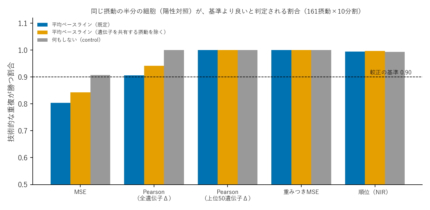
Figure 1. Technical-duplicate win rates against the mean baseline and control.
Table 1. Win rates and DRF in Wessels.
| Metric | Win rate (95% interval) | Median DRF | Win rate with a mean excluding perturbations sharing a targeted gene |
|---|---|---|---|
| MSE | 0.804 (0.748–0.858) | 0.26 | 0.843 |
| Pearson (all-gene Δ) | 0.906 (0.870–0.939) | 0.33 | 0.942 |
| Pearson (top-50-gene Δ) | 1.000 (1.000–1.000) | 0.97 | 1.000 |
| Weighted MSE | 1.000 (1.000–1.000) | 0.93 | 1.000 |
| Rank (NIR) | 0.995 (0.989–0.999) | 1.00 | 0.997 |
Intervals come from 5,000 bootstrap resamples at the perturbation level. The 1,610 perturbation–split observations, 161 perturbations times ten splits, are not independent. Resampling 161 perturbations also does not eliminate dependence between perturbations sharing genes. An interval of 1.000–1.000 describes this sample and bootstrap procedure; it does not imply perfect discrimination in a new experiment.
All point estimates except MSE met the prespecified 0.90 threshold. The all-gene Pearson estimate was 0.906, but its interval, 0.870–0.939, crossed 0.90. MSE's median DRF of 0.26 means that the duplicate closed approximately one-quarter of the gap from the mean baseline to the ideal.
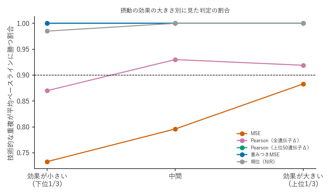
Figure 2. Win rates by tertile of perturbation effect size.
Effect size was the L2 norm of Δ estimated from all cells. MSE win rates increased from 0.733 in the lowest tertile to 0.796 in the middle and 0.883 in the highest. Even the highest tertile remained below 0.90. Weighted MSE, top-gene Pearson and rank were close to 1 in each group.
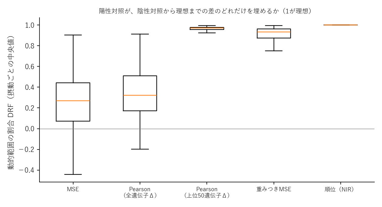
Figure 3. Distribution of DRF across perturbations.
Expected MSE and perturbation-specific signal
Let \(\mu_g\) be the true mean for gene \(g\) under a perturbation, \(\sigma_g^2\) the per-cell variance and \(h\) the number of cells in each half. Assume independent sampling of the two halves, each with mean variance \(\sigma_g^2/h\). The comparison is conditional on a fixed mean-baseline estimate \(m_g\) obtained from other perturbations. The expected sums of squared errors are:
\[ \text{技術的な重複: } 2\sum_g \frac{\sigma_g^2}{h},\qquad \text{平均ベースライン: } \sum_g(\mu_g-m_g)^2+\sum_g\frac{\sigma_g^2}{h}. \]
MSE divides both expressions by the same number of genes. The duplicate therefore has a smaller expected squared error when:
\[ \sum_g(\mu_g-m_g)^2 \;>\; \sum_g\frac{\sigma_g^2}{h}. \]
The perturbation-specific squared deviation must exceed the summed variance of a half-sample mean. Otherwise, the mean baseline has a lower expected MSE. This is an expectation comparison, not a guarantee of the winner in every realized split. Small effects and small cell counts make the duplicate less likely to win, consistent with Figure 2.
After examining the main results, I added an exploratory calculation of this criterion from all-cell estimates, correcting sampling bias in the squared deviation. It agreed with the majority observed outcome for 158 of 161 perturbations, or 98.1%. Always predicting a duplicate win would agree in 80.1%. Because both the criterion and observed outcomes use the same cells, this is not independent validation. It shows consistency with the signal-to-variance explanation.
Two additional datasets
I extended the audit according to an analysis-plan addendum fixed before these calculations. The datasets were Norman (7), comprising 236 combinatorial CRISPRa perturbations in K562 cells, and Replogle K562 essential (8), comprising 1832 single-gene CRISPRi perturbations. A streaming implementation reduced memory use and reproduced all reported Wessels values from the original implementation. Replogle used five random splits because of memory constraints; the other datasets used ten.
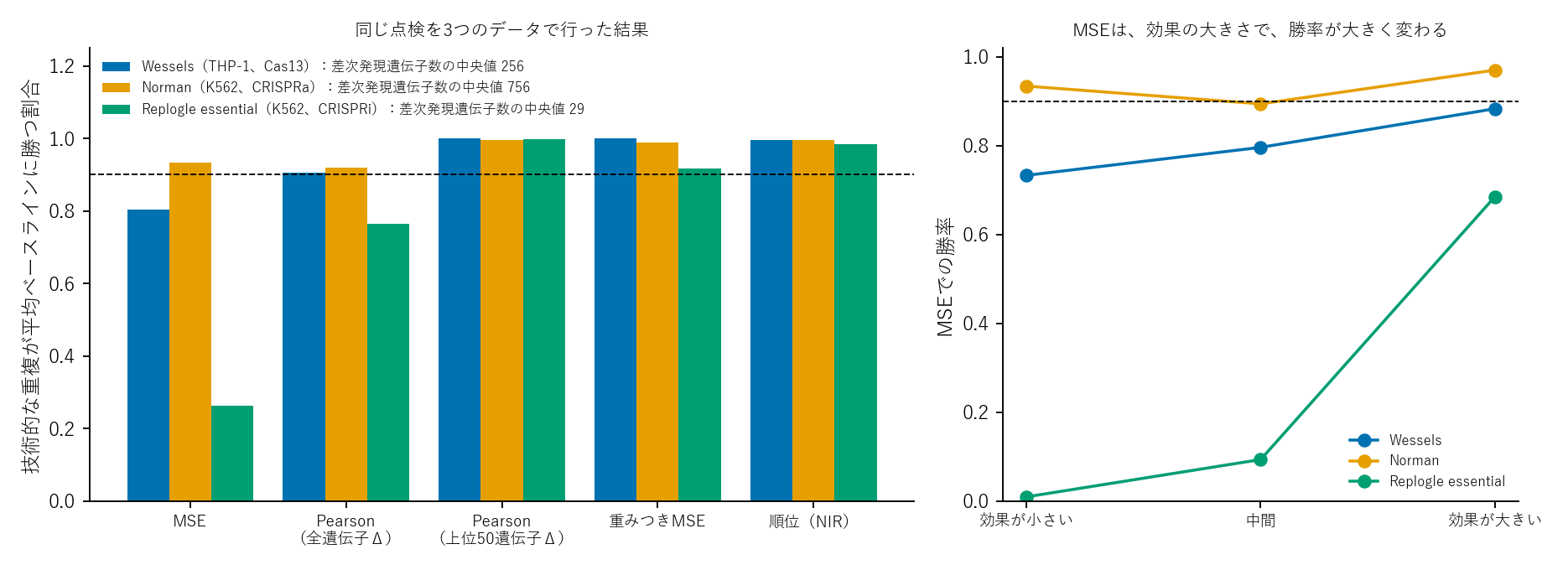
Figure 4. Win rates across three datasets and MSE win rates by effect-size tertile.
Table 2. Win rates across datasets. Intervals are shown for MSE.
| Dataset | Perturbations | Median differentially expressed genes per perturbation | MSE | Pearson (all-gene Δ) | Top 50 genes | Weighted MSE | Rank |
|---|---|---|---|---|---|---|---|
| Replogle essential | 1832 | 29 | 0.262 (0.243–0.282) | 0.764 | 0.997 | 0.917 | 0.984 |
| Wessels | 161 | 256 | 0.804 (0.748–0.858) | 0.906 | 1.000 | 1.000 | 0.995 |
| Norman | 236 | 756 | 0.933 (0.904–0.958) | 0.919 | 0.995 | 0.989 | 0.996 |
A gene was counted as differentially expressed when its Welch-test p value was below 0.05 after Bonferroni correction over the analyzed genes.
MSE win rates differed substantially: 0.26 in Replogle, 0.80 in Wessels and 0.93 in Norman. Their ordering matched the median differential-expression counts, 29, 256 and 756, although no test was performed across only three datasets. Replogle essential's result is directionally consistent with the paper's report that duplicates lose in approximately 95% of perturbations in the larger genome-wide dataset. I did not analyze that genome-wide dataset.
In Replogle, MSE win rates across increasing effect-size tertiles were 0.01, 0.09 and 0.69. Norman's rates were 0.93, 0.89 and 0.97. Weighted MSE, top-gene Pearson and rank exceeded 0.90 in all three datasets. In Replogle, their unrounded win rates were 0.917, 0.997 and 0.984, respectively; all-gene Pearson fell to 0.764.
The exploratory expected-error criterion agreed with the majority outcome in 98.1% of Wessels perturbations, 98.7% of Norman perturbations and 99.1% of Replogle perturbations. Always predicting a win agreed in 80.1%, 94.1% and 26.4%, respectively. Always predicting a loss in Replogle agreed in approximately 74%. These comparisons again reuse the same cells and are not external validation.
The duplicate-versus-mean comparison depends on the dataset's signal and cell counts. A result in one dataset cannot be generalized to another without checking.
Discussion
MSE failed to favor the duplicate in approximately 20% of Wessels perturbations, 74% of Replogle K562 essential perturbations and 7% of Norman perturbations. This supports one premise of Miller and colleagues' argument: the choice of metric can change how superiority over a mean baseline is read. It does not validate their entire model comparison. The alternative metrics exceeded the prespecified threshold in all three datasets, while MSE behavior was consistent with a finite-cell variance explanation.
No predictive model was evaluated here. Discriminating a duplicate from a mean is a different property from correctly ranking models. Biological relevance is a separate question as well. Selecting highly responsive genes or weighting them strongly can structurally favor a perturbation-specific prediction over a global mean. Such discrimination does not establish that a predicted response is biologically correct.
Scope also matters. The larger Replogle K562 GWPS dataset, approximately 8.8 GB, was not analyzed. The paper reports approximately 95% duplicate losses there in its Extended Data Fig. 1e, relating this to signal dilution: a reported mean of 3.25 differentially expressed genes per perturbation versus 102 in Norman19. Those paper-reported means should not be equated with my differently defined median of 29 in Replogle essential.
Limitations
The datasets use specific cell lines and interventions: THP-1 Cas13 combinatorial perturbations for Wessels, K562 combinatorial CRISPRa for Norman, and K562 single-gene CRISPRi for Replogle. Many Wessels perturbations share genes such as INTS1, strengthening the mean baseline. Excluding shared-target perturbations increased win rates without changing the main interpretation. This sensitivity analysis does not apply to Replogle's single-gene interventions. Replogle used five splits rather than ten.
Splitting cells increases the variance of the duplicate mean and can disadvantage it under MSE. That is a property of this technical-duplicate construction, also defined in Miller and colleagues' paper, rather than evidence that the reference is noise-free. Top-50-gene selection and differential-expression weights use all cells and are not independent of the reference. Pearson correlation is undefined for the control prediction's zero-change vector; I assigned it 0.
The main cell splits and metric calculations were unchanged. The DRF column, exploratory expected-error criterion and bootstrap intervals were added during examination and review after the main results were available; the original values remained unchanged. An independent implementation using seed 777 and 20 splits produced MSE and all-gene Pearson win rates of 0.801 and 0.910. This reviewer recalculation checks implementation on the same underlying cells, rather than providing new experimental replication.
Data and code availability
The analysis ZIP contains the plan, cross-dataset addendum, code, results and figure-generation code. Original data are not redistributed; download scripts and SHA-256 hashes are included.
For Wessels, run python fetch_data.py && python analysis.py && python figures.py. The download is approximately 219 MB; dependencies are numpy, scipy, anndata and matplotlib. The recorded run took approximately three minutes with a fixed seed.
For Norman and Replogle, run python fetch_data.py all, downloading approximately 0.7 GB and 1.5 GB, followed by python analysis_stream.py data/raw/NormanWeissman2019_filtered.h5ad control norman and python analysis_stream.py data/raw/ReplogleWeissman2022_K562_essential.h5ad control replogle_essential 5. The streaming calculation also reproduces Wessels results with python analysis_stream.py data/raw/WesselsSatija2023.h5ad control wessels_stream.
References
- Ahlmann-Eltze C, Huber W, Anders S. Deep-learning-based gene perturbation effect prediction does not yet outperform simple linear baselines. Nature Methods. 2025;22(8):1657–1661. doi:10.1038/s41592-025-02772-6.
- Miller HE, Mejia GM, Leblanc FJA, Swain B, Wang B, de Lima Camillo LP. Deep learning perturbation models can outperform baselines on calibrated metrics. Nature Biotechnology. 2026 Oct 1. Published online. doi:10.1038/s41587-026-03307-w.
- Kumakura D. What did the Virtual Cell predict? Target genes and evaluation shortcuts. 2026 Oct 11. Article.
- Wessels HH, Méndez-Mancilla A, Hao Y, Papalexi E, Mauck WM, Lu L, et al. Efficient combinatorial targeting of RNA transcripts in single cells with Cas13 RNA Perturb-seq. Nature Methods. 2023;20(1):86–94. doi:10.1038/s41592-022-01705-x.
- Peidli S, Green TD, Shen C, Gross T, Min J, Garda S, et al. scPerturb: harmonized single-cell perturbation data. Nature Methods. 2024;21(3):531–540. doi:10.1038/s41592-023-02144-y.
- Peidli S, Green TD, Shen C, Gross T, Min J, Garda S, et al. scPerturb Single-Cell Perturbation Data: RNA and protein h5ad files [Dataset]. Version 1.4. Zenodo; 2022. doi:10.5281/zenodo.13350497.
- Norman TM, Horlbeck MA, Replogle JM, Ge AY, Xu A, Jost M, et al. Exploring genetic interaction manifolds constructed from rich single-cell phenotypes. Science. 2019;365(6455):786–793. doi:10.1126/science.aax4438.
- Replogle JM, Saunders RA, Pogson AN, Hussmann JA, Lenail A, Guna A, et al. Mapping information-rich genotype-phenotype landscapes with genome-scale Perturb-seq. Cell. 2022;185(14):2559–2575.e28. doi:10.1016/j.cell.2022.05.013.