Combination perturbations: how much remains beyond additivity?
A K562 CRISPRa reanalysis estimates nonadditive expression components, distinguishing response scaling, sampling noise and model-evaluation headroom.
On this page
Models such as GEARS predict cellular responses to simultaneous perturbations from single-perturbation information (1). Additive expression-change predictions are a common comparator. Ahlmann-Eltze and colleagues report that deep learning has not yet surpassed simple linear baselines, including additivity (2). How much room is there to improve on that baseline?
I estimated nonadditive expression-change components in Norman et al.'s public two-gene CRISPRa data (3), separating sampling noise under the stated assumptions. This does not evaluate a particular predictive model.
Question and intended use
The question is how much simultaneous two-gene CRISPRa expression change remains beyond the sum of single changes after accounting for noise. The intended use is interpreting combination-prediction evaluations and their potential headroom, not measuring a model's performance.
Data
Norman et al. activate single genes or pairs in K562 leukemia cells and measure individual-cell RNA with Perturb-seq. CRISPRa activates target transcription rather than knocking genes out. I use the scPerturb release (4), publicly accessible under CC BY 4.0: 111,445 cells, 105 single perturbations, 131 pairs and 11,855 controls. Both single perturbations exist for every pair.
Methods
Counts are normalized to 10,000 per cell and transformed with log1p, the natural logarithm after adding one. The analysis uses 7,812 genes detected in at least 10% of all cells. Perturbation changes are mean expression minus the control mean. Additivity sums A and B changes on this log-transformed scale; summing untransformed expression would define another baseline.
Double-perturbation cells are randomly split into three fixed-seed groups. The first selects the 50 largest-changing genes, avoiding selection on the same sampling noise used for evaluation. Activated targets A and B are excluded after an initial analysis revision; changes before and after revision are reported below. At least one target was absent from the initial 7,812-gene set in 97 of 131 pairs. The other two groups provide nonoverlapping cell observations within the same experiment, not independent biological replicates.
The nonadditive fraction F multiplies each observation's residual from the additive prediction and divides by the cross-product of observed changes. Independent mean-zero observation errors cancel in expectation in the cross-product. F=0 represents additivity; F=0.2 describes a nonadditive squared-change component equal to 20% of the squared change norm, not 20% of genes. Estimates can exceed one when residuals exceed total change or become negative through noise.
A one-coefficient comparison multiplies the additive prediction by c, fitted using the first split independently of the evaluation groups. c<1 attenuates the sum and c>1 amplifies it. I also fit separate coefficients c1 and c2 for A and B, as in Norman et al.; the single-coefficient form constrains c1=c2. The original study uses these coefficients among other information to classify synergy, suppression and dominance. This analysis revisits those patterns quantitatively.
The reported R² uses squared change norm as denominator. It is not the usual gene-mean-centered R². One denotes perfect prediction. The plan was fixed before calculation. Post-result additions include correction for single-perturbation prediction noise, summaries of c and exploratory interpretations of pairs such as those containing CEBPE.
Median nonadditivity is small
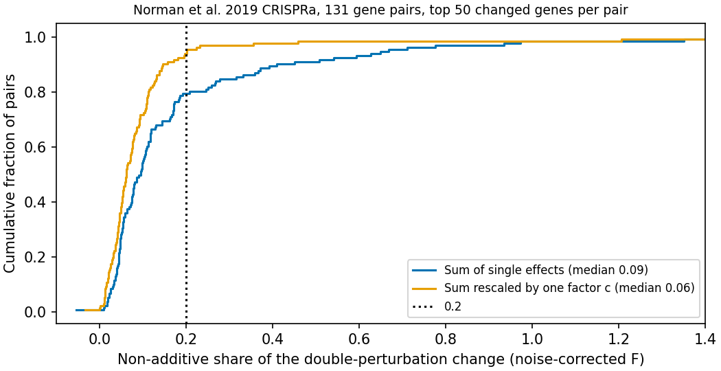
Figure 1. F across 131 pairs. Blue uses unscaled additivity; orange scales it with one coefficient.
Table 1. Nonadditivity and additive-prediction summaries, excluding target genes.
| Metric, top 50 genes excluding targets | Value |
|---|---|
| Median F, interquartile range | 0.09 (0.05–0.17) |
| Pairs with F >0.2 | 27 (21%) |
| Median F after one coefficient | 0.06 |
| Pairs with F >0.2 after one coefficient, among all 131 | 8 |
| Median F after two coefficients, Norman form | 0.05 |
| Median F after single-perturbation noise correction, post hoc | 0.08 |
| Median additive R², including noise | 0.89 |
| Median R² between two observation groups | 0.96 |
The prespecified rule calls headroom small when median F<0.2. The result meets that rule. Interquartile range means the 25th–75th percentiles. Additive R² of 0.89 versus within-experiment agreement between splits of 0.96 gives an orienting gap, not a universal model ceiling.
Excluding target genes changed median F from 0.090 to 0.094, left the count above 0.2 at 27, and changed scaled median F from 0.047 to 0.061. Moving coefficient estimation to the first split also contributes to the last change.
Four split seeds including the main analysis gave median F 0.08–0.09. Using top 20 or 200 genes gave 0.09; excluding three low-agreement pairs with R²<0.5 also gave 0.09. Across all 7,812 genes F rose to 0.21. Halving single-perturbation cell counts increased F, allowing a post hoc correction for that prediction-noise bias; corrected F was 0.13. Including small-change genes therefore increases estimated nonadditivity somewhat.
Large deviations often concern response magnitude
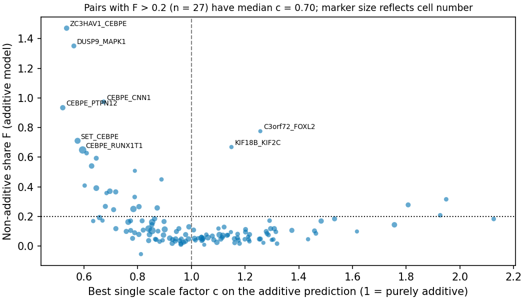
Figure 2. Coefficient c against F for 131 pairs; point area represents cell count.
Table 2. The 27 pairs with F>0.2, ordered by F.
| Pair | Cells | F | c | F after one coefficient | R² between observation groups |
|---|---|---|---|---|---|
| ZC3HAV1 + CEBPE | 410 | 1.47 | 0.54 | 0.106 | 0.91 |
| DUSP9 + MAPK1 | 290 | 1.35 | 0.56 | 0.121 | 0.81 |
| CEBPE + CNN1 | 237 | 0.97 | 0.67 | 0.223 | 0.92 |
| CEBPE + PTPN12 | 415 | 0.93 | 0.52 | 0.090 | 0.95 |
| C3orf72 + FOXL2 | 59 | 0.78 | 1.26 | 1.825 | 0.50 |
| SET + CEBPE | 658 | 0.71 | 0.58 | 0.113 | 0.99 |
| KIF18B + KIF2C | 96 | 0.67 | 1.15 | 1.205 | -0.16 |
| CEBPE + RUNX1T1 | 1219 | 0.65 | 0.59 | 0.041 | 0.99 |
| CEBPE + CEBPA | 180 | 0.63 | 0.61 | 0.015 | 0.97 |
| MAP2K6 + SPI1 | 302 | 0.59 | 0.65 | 0.124 | 0.94 |
| CEBPE + KLF1 | 468 | 0.54 | 0.63 | 0.202 | 0.96 |
| CEBPB + CEBPA | 64 | 0.51 | 0.79 | 0.107 | 0.87 |
| CDKN1B + CDKN1A | 134 | 0.45 | 0.89 | 0.232 | 0.88 |
| IGDCC3 + PRTG | 140 | 0.41 | 0.60 | 0.001 | 0.81 |
| MAP2K3 + MAP2K6 | 571 | 0.39 | 0.65 | 0.025 | 0.95 |
| MAPK1 + PRTG | 500 | 0.37 | 0.70 | 0.196 | 0.97 |
| IGDCC3 + MAPK1 | 368 | 0.37 | 0.72 | 0.142 | 0.95 |
| CDKN1C + CDKN1A | 126 | 0.36 | 0.68 | -0.001 | 0.91 |
| LYL1 + CEBPB | 192 | 0.33 | 0.79 | 0.172 | 0.93 |
| FEV + CBFA2T3 | 159 | 0.32 | 1.95 | 0.156 | 0.96 |
| PTPN12 + UBASH3A | 311 | 0.28 | 1.81 | 0.117 | 0.97 |
| PTPN12 + OSR2 | 339 | 0.27 | 0.68 | 0.091 | 0.86 |
| FOSB + UBASH3B | 426 | 0.27 | 0.80 | 0.130 | 0.92 |
| ETS2 + IGDCC3 | 441 | 0.26 | 0.87 | 0.180 | 0.95 |
| UBASH3B + OSR2 | 796 | 0.25 | 0.78 | 0.138 | 0.95 |
| CEBPB + PTPN12 | 331 | 0.25 | 0.71 | 0.076 | 0.94 |
| CNN1 + UBASH3A | 178 | 0.21 | 1.93 | 0.195 | 0.95 |
Both c and scaled F use c fitted on the first split. Scaling can worsen held-out F when few cells or weak changes make estimation unstable, as for C3orf72+FOXL2 and KIF18B+KIF2C.
Of these 27 pairs, 22 have c<1; their post hoc median c is 0.70. Many largely preserve change direction while attenuating magnitude. Two-coefficient fits additionally reveal attenuation of one contribution: for ZC3HAV1+CEBPE, coefficients are 0.96 and 0.46, respectively. This includes patterns resembling the original dominance category, beyond uniform attenuation. Three pairs have c>1.8: FEV+CBFA2T3, PTPN12+UBASH3A and CNN1+UBASH3A.
Five of the 27 remain above F=0.2 after one coefficient, so 22 fall below it. These are not necessarily the same 22 with c<1. Three originally below 0.2 instead rise above it, giving eight among all 131. C3orf72+FOXL2 has only 59 cells and scaled F=1.83 versus unscaled 0.78. KIF18B+KIF2C has between-split R²=−0.16; its underlying change is poorly measured. C3orf72+FOXL2 has agreement 0.50. Such small-cell or weak-change estimates are unreliable.
Seven of the 27 pairs contain the granulocytic-differentiation transcription factor CEBPE. Its large single-perturbation response tends to weaken in combinations. This exploratory observation cannot distinguish biological interaction from guide efficiency or changed differentiation-state composition. Across all 131 pairs, median c is 0.99, interquartile range 0.82–1.19; 22% have c<0.8. Both attenuation and amplification occur.
Interpreting predictive-model evaluations
Additivity is a strong comparator here: it explains approximately 90% of squared response change at the median. A model improvement operates within the remaining component. Placing that gain alongside within-experiment agreement between splits makes its scale clearer.
Much of the large residual concerns magnitude, either uniform scaling or attenuation of one single-perturbation contribution. Predicting which combinations scale differently is therefore a concrete challenge, consistent with Norman et al.'s coefficient-based classification.
Noise treatment and gene selection change the result. Selecting and evaluating genes on the same cells, including all genes, or retaining the activated targets can increase apparent nonadditivity. They define different evaluation tasks and must be specified.
Limitations
- K562 CRISPRa results do not establish behavior under knockout, inhibitors, drug combinations or other cell types. Activation strengths vary by guide and may weaken in double perturbations.
- The 131 pairs were selected by the original investigators to study interactions, not sampled randomly.
- Additivity is defined on log-transformed expression. c<1 can reflect technical effects such as expression saturation.
- Only RNA changes are evaluated, not growth, survival or synthetic lethality.
- The smallest condition has 54 cells, leaving 18 per split. Pair-specific confidence intervals were not calculated.
Implementation checks
An independent implementation for 12 pairs used scanpy normalization and dense-matrix means. F agreed through five decimal places. It reimplemented the same splitting rule, so cannot detect an error in that rule itself. Four synthetic checks cover noise inflation, recovery of nonadditive fraction, correct splitting and F=0/c=1 under exact additivity. Fixed-seed reruns produce byte-identical result files; input hashes use SHA-256.
Data and code availability
Run python acquire.py && python test_analysis.py && python analysis.py && python figures.py && python validate.py. The environment uses Python 3.12, anndata, scanpy, numpy, scipy, pandas, matplotlib and requests. The companion archive includes the plan, code, acquisition instructions, checksums, results and validation outputs.
References
- Roohani Y, Huang K, Leskovec J. Predicting transcriptional outcomes of novel multigene perturbations with GEARS. Nature Biotechnology. 2024;42(6):927-935. doi:10.1038/s41587-023-01905-6.
- Ahlmann-Eltze C, Huber W, Anders S. Deep-learning-based gene perturbation effect prediction does not yet outperform simple linear baselines. Nature Methods. 2025;22(8):1657-1661. doi:10.1038/s41592-025-02772-6.
- Norman TM, Horlbeck MA, Replogle JM, Ge AY, Xu A, Jost M, et al. Exploring genetic interaction manifolds constructed from rich single-cell phenotypes. Science. 2019;365(6455):786-793. doi:10.1126/science.aax4438.
- Peidli S, Green TD, Shen C, Gross T, Min J, Garda S, et al. scPerturb: harmonized single-cell perturbation data. Nature Methods. 2024;21(3):531-540. doi:10.1038/s41592-023-02144-y. Data: Zenodo, CC BY 4.0.