Designing the data for virtual cells: a synthetic allocation audit inspired by Biohub
Four synthetic allocations of 28,800 cells separate sampling depth, donors, condition coverage, imputation bias, and sample-preparation costs.
On this page
- Introduction
- Put the prediction target into a measurement-design table
- Allocate the same cells to depth, breadth, and replication
- More cells reduce one source of error but leave another
- What fills the unmeasured combinations?
- Equal cell totals do not mean equal sample-preparation burdens
- Discussion
- Data and code availability
- References
Introduction
“Measure more cells, and we will be able to predict responses to cellular interventions.” Before starting those measurements, one question deserves attention: should we add cells under the same conditions, independent donors, or combinations of conditions that have not yet been measured?
On October 7, 2026, Biohub announced an expansion of its Virtual Biology Initiative. Collaboration with DOE, NIH, and other partners aims to build the data and measurement technologies underlying models of cellular responses to interventions. Shared standards, common identifiers, and data access are part of the plan (1, 2).
This is a program to build the foundation for models, not a report of a completed universal cell model. That makes measurement design consequential. I constructed four synthetic allocations of the same 28,800 cells. The calculations do not reproduce Biohub's data or budget; they make concrete the choices that precede training-data generation.
Put the prediction target into a measurement-design table
Suppose the goal is to estimate RNA responses to perturbations across cellular backgrounds and time points. Here the target is the donor-population mean treatment–control difference for each of 4 backgrounds × 6 perturbations × 3 times, or 72 combinations. All combinations receive equal evaluation weights.
This does not predict an individual cell's future or a new patient's response. Mean RNA changes also do not necessarily establish protein function or disease improvement. Additional modalities, if needed, belong in the design, but this example studies one response quantity and does not estimate the benefit of adding modalities.
The table records measured combinations, donor correspondence, and model-imputed conditions separately from total cell count. Generalization to a new background or perturbation type requires withholding that axis explicitly. Here every level of background, perturbation, and time is represented in training; only some combinations are unmeasured.
Allocate the same cells to depth, breadth, and replication
The four designs are fixed. Cell counts below refer to one treatment or control arm for each condition and donor. Totals include both arms.
Table 1. Four allocations with equal total cell counts.
| Design | Measured combinations | Donors | Cells per arm | Total cells including both arms |
|---|---|---|---|---|
| Depth | 18 | 2 | 400 | 28,800 |
| Breadth | 72 | 2 | 100 | 28,800 |
| Replication | 36 | 8 | 50 | 28,800 |
| Balanced | 72 | 4 | 50 | 28,800 |
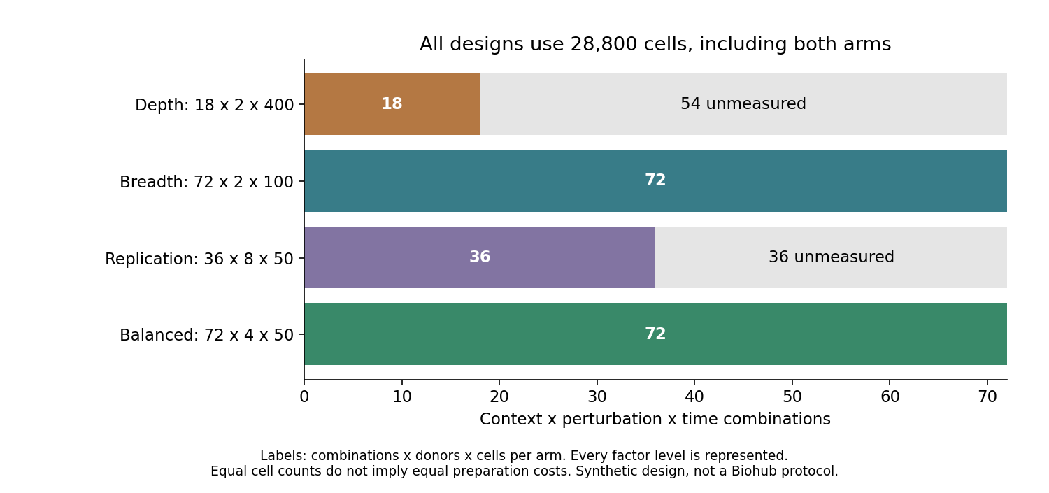
Figure 1. Gray indicates unmeasured combinations. Every design contains all background, perturbation, and time levels; the comparison does not withhold an entire perturbation. Labels show combinations × donors × cells per arm, not equal financial costs.
Even the 18-condition design includes combinations sufficient to estimate additive background, perturbation, and time effects. Each additive design matrix has 11 columns and full rank. Representing every level and having full rank do not identify condition-specific responses beyond additivity.
More cells reduce one source of error but leave another
Each condition's response is estimated from donor-level treatment–control differences. Let \(\tau\) be the standard deviation of donor-by-condition response differences and \(\sigma\) the cell-noise standard deviation in each arm. With \(D\) donors and \(c\) cells per arm, the variance of the direct mean is
\[ \operatorname{Var}(\widehat{\Delta}) =\frac{\tau^2}{D}+\frac{2\sigma^2}{Dc} \]
The factor of 2 reflects independent cell measurements in the two arms. Increasing \(c\) reduces the second term; deeper measurement of the same donors leaves the first term.
For example, assuming \(\tau=\sigma=1\), two donors with 50 cells per arm give a standard error of 0.721. Increasing cell recovery eightfold to 400 per arm lowers it only to 0.709. Four donors with 50 cells per arm give 0.510. These values are calculated in response units under assumptions, not measured biological errors.
When donor variation is absent, increasing cell counts has greater relative value. These results do not support universally prioritizing donors over cells. That judgment requires separate estimates of donor variation, measurement noise, and recovery by cell type from prior data.
The formula also assumes independent donor response differences across conditions. Reusing a donor across conditions can introduce correlated responses and alter predictive covariance. That assumption must be checked when connecting the calculation to an actual experiment.
What fills the unmeasured combinations?
The true mean response consists of additive background, perturbation, and time components plus a condition-specific nonadditive component. One might imagine a perturbation working only in one background at a late time, beyond the sum of effects along each axis. The pattern here is not estimated from a real phenomenon: it is generated with a fixed random seed, orthogonalized to the additive component, and normalized to root mean square 1 across all 72 conditions. Its strength \(\lambda\) takes values 0, 0.5, 1, and 2. Designs are not reselected using the truth. Cell-noise standard deviation remains \(\sigma=1\) in every comparison.
The estimator is identical across designs. A measured combination uses its direct mean. Only unmeasured combinations use predictions from an additive least-squares model fitted to measured conditions. This simple illustrative rule is not a comparison of trained foundation models.
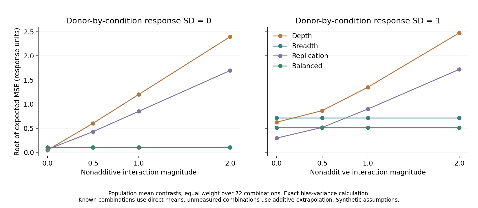
Figure 2. The vertical axis is the square root of mean expected squared error over all 72 conditions, calculated exactly from bias and variance. It is not a biological confidence interval from independent experiments. Breadth and Balanced overlap in the left panel because their values coincide.
Table 2. Expected error with donor variation \(\tau=1\).
| Design | No nonadditive component, \(\lambda=0\) | Nonadditive component present, \(\lambda=1\) |
|---|---|---|
| Depth | 0.622 | 1.350 |
| Breadth | 0.714 | 0.714 |
| Replication | 0.294 | 0.896 |
| Balanced | 0.510 | 0.510 |
When additivity is correct, measuring 36 conditions in eight donors efficiently predicts unmeasured conditions and gives the smallest error among these four designs. With nonadditivity, however, imputation becomes biased. At \(\lambda=1\), measuring all 72 conditions in four donors gives the smallest error.
Breadth and Balanced have horizontal curves because the estimator directly measures every condition and never imputes its nonadditive component. This does not mean every model attains this performance merely by adding conditions. An estimator that predicts everything using only an additive model retains nonadditive error even when all conditions have been measured.
I also generated 2,000 synthetic experiments and compared empirical means with exact expected squared errors. Across 48 settings, comprising four designs × three donor-variation levels × four nonadditive strengths, the largest discrepancy was approximately 1.53 Monte Carlo standard errors. This checks implementation, not biological assumptions.
The ranking depends on one fixed nonadditive pattern, four designs, one estimation rule, and equal evaluation weights. Errors on unmeasured combinations are separately provided in the output tables; they are undefined for designs with no unmeasured conditions. A score including measured conditions is not an unseen-condition generalization score. If one cellular background dominates the intended use, evaluation weights and the design require reconsideration.
Equal cell totals do not mean equal sample-preparation burdens
Counting each condition, donor, and treatment/control arm separately gives 72 samples for Depth, 288 for Breadth, and 576 each for Replication and Balanced. This assumes no shared controls or pooling and does not generalize actual library counts.
Suppose preparing each sample adds a cost equivalent to measuring 100 cells. Combined cell and sample costs become 36,000, 57,600, 86,400, and 86,400 cell equivalents, respectively. These are not prices. The sensitivity calculation shows why fixed sample costs invalidate an equal-budget interpretation of equal cell totals. Output tables also cover fixed costs of 0, 25, 100, and 400 cell equivalents.
Real costs include donor acquisition, culture and perturbation success, tissue and cell-type recovery, multimodal measurement, instrument time, and quality control. This calculation does not optimize a fixed monetary budget.
Discussion
The Biohub initiative combines data scale with technologies for measuring interventions and infrastructure connecting measurements. Its April launch also described expanding measurement across molecular, spatial, and dynamic dimensions (3).
The calculation separates noise reduced by deeper measurement, variability reduced by additional donors, and imputation bias avoided by broader condition coverage. Their relative importance changes prediction error even at identical cell totals.
This remains a comparison under fixed hypothetical conditions, not an estimate of optimal allocation for actual Biohub data. More cells in measured conditions cannot by themselves supply missing combinations of backgrounds, perturbations, times, and donors.
Data and code availability
The analysis code, settings, output tables, and original figures can be downloaded. Python and NumPy run the calculations and 10 tests; redrawing figures also requires Matplotlib.
All inputs are original synthetic settings. The distribution contains no actual data, original-paper figures, third-party code, or internal Biohub plans. REPRODUCE.md and the code document settings, randomness, estimands, unmeasured-condition definitions, and cost assumptions. Results illustrate experimental-design reasoning; they do not validate foundation-model performance, an optimal donor count, or clinical usefulness.
References
- Biohub. International, cross-sector collaboration commits nearly $2 billion to build foundational data for AI models to predict and treat disease. 2026 Oct 7. Announcement.
- US Department of Energy. DOE, NIH, and Biohub Partner to Build Foundational Data for Predictive Biological Super Intelligence Models. 2026 Oct 7. Announcement.
- Biohub. Biohub Launches the Virtual Biology Initiative to Galvanize a Global Effort to Create the Open Data Foundation for AI-Accelerated Biology. 2026 Apr 29. Announcement.