PK/PD, population PK, PBPK and QSP: purposes, data and interpretation
On this page
- Abstract
- Introduction
- PK, PD and overlapping model categories
- PK/PD: concentration and response over time
- PopPK: explaining concentration differences
- PBPK: physiological determinants of concentration
- QSP: connecting drug action and biological systems
- Structure, variability and estimation are separate axes
- Discussion
- Conclusion
- Data and code availability
- References
Abstract
PK/PD, PopPK, PBPK and QSP describe overlapping aspects of drug modeling, rather than successive levels of sophistication. Foundational literature, reviews and guidance are compared in terms of questions, inputs, outputs and interpretation. Synthetic examples show different response profiles under the same PK and conditional concentration variability under assumed clearance distributions. Model structure, representation of variability and estimation framework are separate choices. Credibility depends on observations, assumptions and intended use, rather than the model name.
Literature checked on October 9, 2026. Figures are original conceptual diagrams or simulations of a hypothetical drug.
Introduction
PK/PD, PopPK, PBPK and QSP all appear in discussions of doses and effects, often using differential equations. They can look like different names for similar models.
The names do not share one classification axis. PK/PD links dosing, exposure and response; PopPK addresses population pharmacokinetics and individual variability; PBPK represents pharmacokinetics using physiology; QSP quantitatively connects drug action with biological systems. They overlap and can be linked. They are not four steps from simple to advanced.
This article compares purposes, input data and interpretation as well as definitions. It is a guide to reading analysis plans and reports, not a complete implementation manual.
PK, PD and overlapping model categories
Pharmacokinetics (PK) describes drug concentrations over time against absorption, distribution, metabolism and excretion (ADME). The relevant concentration may be plasma, whole blood, tissue or unbound drug, depending on the question.
Pharmacodynamics (PD) addresses exposure–action or exposure–response relationships, including receptor occupancy, biomarkers, tumor changes and adverse effects. Target occupancy is not clinical benefit.
“What the body does to the drug” versus “what the drug does to the body” is a useful introduction, but drug-induced physiological changes can also alter PK. The connection need not be one-way (1).
Table 1. Terms and their principal emphasis
| Term | Meaning | Main emphasis |
|---|---|---|
| PK/PD, also PKPD or PK-PD | Pharmacokinetic/pharmacodynamic modeling | Dosing, concentration, response and time |
| PopPK | Population pharmacokinetics | Typical PK, variability and covariates |
| PBPK | Physiologically based pharmacokinetic modeling | Concentrations through organs, blood flow, metabolism and transport |
| QSP | Quantitative systems pharmacology | Interactions among drug action, pathways, cells, regulation and disease |
This is not an exclusive taxonomy. PBPK can connect to PD, and QSP can use a conventional PK exposure model.
Table 2. Questions, inputs and outputs
| Approach | Main purpose | Example inputs | Example outputs |
|---|---|---|---|
| PK/PD | Exposure–response, delays and dosing effects | Dose history, concentrations, timed biomarkers/efficacy/safety | Exposure–response relationships, response trajectories and uncertainty |
| PopPK | Explain concentration variability and compare exposure/regimens | Individual dose and sampling times, concentrations, weight, organ function and concomitant drugs | Typical CL/V, variability, covariates and exposure distributions |
| PBPK | Predict exposure under altered physiology or interactions | Physicochemical properties, binding, enzyme/transporter experiments, physiology and clinical PK | Blood/tissue concentrations, interaction ratios, predictions and sensitivity |
| QSP | Examine disease–drug interactions, combinations and response heterogeneity | Binding/pathway/cell experiments, disease biology, PK, biomarkers and clinical outcomes | Mechanistic hypotheses, response dynamics, virtual-population results and sensitivity |
These are examples, not universally mandatory inputs. Individual observations differ from aggregate summaries; in vitro information differs from clinical evidence; construction and verification data require separate roles.
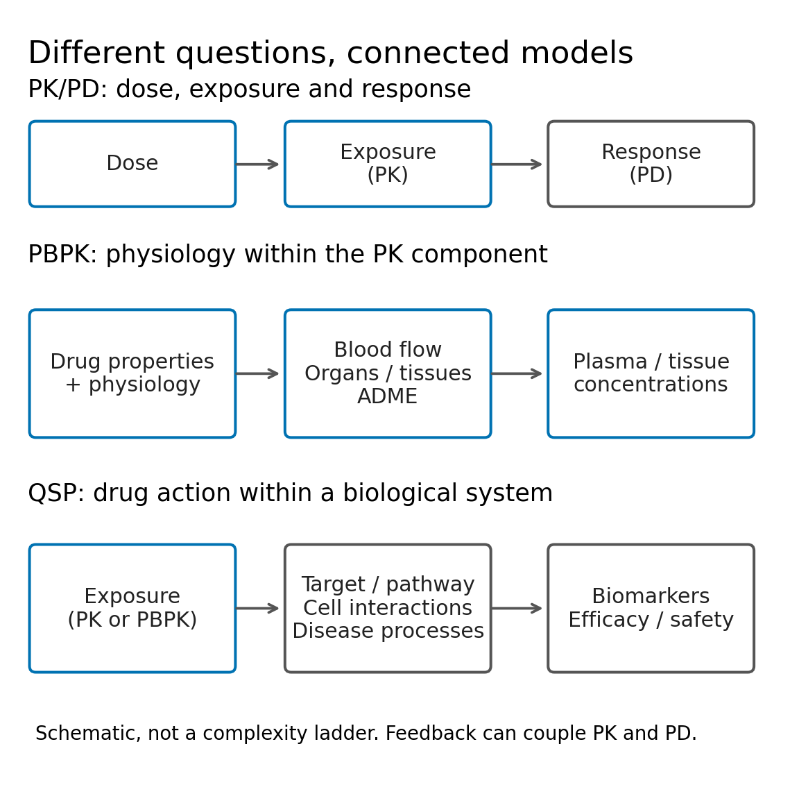
Figure 1. Modeling emphases. The top row shows dosing to response, and the lower rows show principal biological representations. Vertical order denotes neither superiority nor exact set inclusion. PK and PD can interact, as with target-mediated elimination. PopPK variability is treated as a separate axis overlaid on PK structure (Figure 3).
PK/PD: concentration and response over time
Purpose and data
Questions include whether equal total doses at different intervals change response and why biomarkers peak after concentration. Alongside dose history and PK, response measurement times, baseline values and covariates matter. Responses can be continuous values, events or event times.
Corresponding PK and PD within the same participants support within-person relationships. Connecting separate trials or aggregate values adds assumptions about populations and measurements. Sequential PK-then-PD estimation and simultaneous estimation are alternatives; sequential approaches require consideration of PK uncertainty propagation.
Direct and delayed response examples
After one intravenous bolus, a one-compartment model gives
\[ C(t)=\frac{D}{V}\exp\left(-\frac{CL}{V}t\right) \]
Here \(D\) is dose, \(V\) volume and \(CL\) clearance. The assumptions are instantaneous IV dosing, constant parameters and linear elimination. The compartment need not be an anatomical organ.
Connect a saturating response:
\[ E(C)=\frac{C}{EC_{50}+C}. \]
Maximum response is one in this example; \(EC_{50}\) gives half that maximum. With immediate response, \(E(C(t))\) is the response trajectory. Production and removal delays can instead produce a later peak (2).
For normalized change from baseline, consider
\[ \frac{dR}{dt}=k_{\mathrm{out}}\{E(C(t))-R\},\qquad R(0)=0 \]
This can represent normalized drug-stimulated turnover; it is not assigned directly to occupancy or clinical effect. If a quantity \(B\) follows \(dB/dt=k_{\mathrm{in}}\{1+sE(C)\}-k_{\mathrm{out}}B\), with baseline \(B_0=k_{\mathrm{in}}/k_{\mathrm{out}}\) and stimulation magnitude \(s>0\), transforming \(R=(B/B_0-1)/s\) yields this equation. Thus \(R=0\) means no change from baseline, not zero substance or physiological response. The delay follows turnover and initial conditions, not merely a horizontal shift.
The hypothetical parameters were dose 100 mg, volume 10 L, clearance 1 L/h, \(EC_{50}=2\) mg/L and \(k_{\mathrm{out}}=0.05\) h\(^{-1}\).
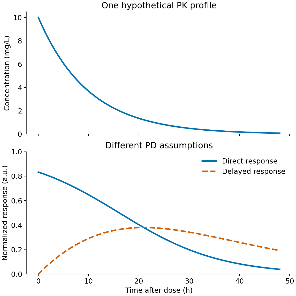
Figure 2. Same PK under different PD assumptions. Responses over 0–48 hours are normalized arbitrary units. This is neither fitting observations nor predicting an actual drug. model_demo.py produces results/trajectories.csv and results/summary.json.
Table 3. Response peaks in the synthetic example
| Response assumption | Peak time | Maximum response, arbitrary units |
|---|---|---|
| Immediate concentration response | 0.00 h | 0.833 |
| Turnover delay | 20.95 h | 0.381 |
Times use a 0.05-hour grid. PD assumptions alone change magnitude and timing; observations and biology are needed to choose between them.
PK/PD can include delays and physiological mechanisms. Contrasting it as mere curve fitting with mechanistic QSP misses the continuum between mechanism-based PK/PD and systems models.
Interpretation and limits
Fit is only one consideration. Peak timing, recovery, repeated-dose accumulation and history dependence matter, as do concentration ranges supporting separate EC50/maximum-effect estimates and sampling times distinguishing delays. Different equations can fit similarly over narrow doses.
Exposure association does not guarantee the causal effect of changing exposure. Disease may alter clearance and outcomes simultaneously; discontinuation, missingness and concomitant therapy also matter. Biomarker improvement is not an unvalidated clinical benefit.
PopPK: explaining concentration differences
Purpose and data
PopPK estimates typical population PK and variability. Questions concern exposure changes with covariates, variability under a regimen, and how individual samples inform that person's PK (3).
Concentrations must remain linked to participant, dose and sampling time.
Table 4. Data needed for population analysis
| Data | Preanalysis question |
|---|---|
| Participant, study, arm and visit identifiers | Can within-person repetition be separated from between-person variability? |
| Actual dose, route, time and infusion duration | How are interruptions, deviations and adherence represented? |
| Sampling times, concentrations, units and assays | Are times and values aligned, units harmonized and samples comparable? |
| Weight, organ function, concomitant drugs and background | Which timepoint supplies each covariate, including time-varying values? |
| Below-quantification values, missingness and exclusions | What supports their treatment without equating undetected values with zero? |
Sparse individual data can be informative if population-wide sampling covers needed times. Trough-only sampling still poorly identifies absorption or distribution rates. PopPK does not make every parameter identifiable from sparse data.
Structure, covariates and variability
An example nonlinear mixed-effects model writes individual clearance as
\[ CL_i=CL_{70}\left(\frac{WT_i}{70\ \mathrm{kg}}\right)^\theta\exp(\eta_i),\qquad \eta_i\sim N(0,\omega^2) \]
\(CL_{70}\) is the reference typical value, \(WT_i\) weight, \(\theta\) the weight coefficient and \(\eta_i\) unexplained individual variability. Under this lognormal example, the typical value is the conditional median, not necessarily the arithmetic mean.
Residuals capture variation beyond individual PK. A proportional example is \(Y_{ij}=C_i(t_{ij})(1+\varepsilon_{ij})\), but suitable error structure depends on concentration range and assay. Between-person, between-occasion and residual variation differ. Residuals can include model omissions and uncertain dose times as well as assay error.
For illustration, assume weight exponent 0.75, \(CL_{70}=1\) L/h and \(\omega=0.25\), using the same hypothetical 100 mg dose and fixed \(V=10\) L as Figure 2.
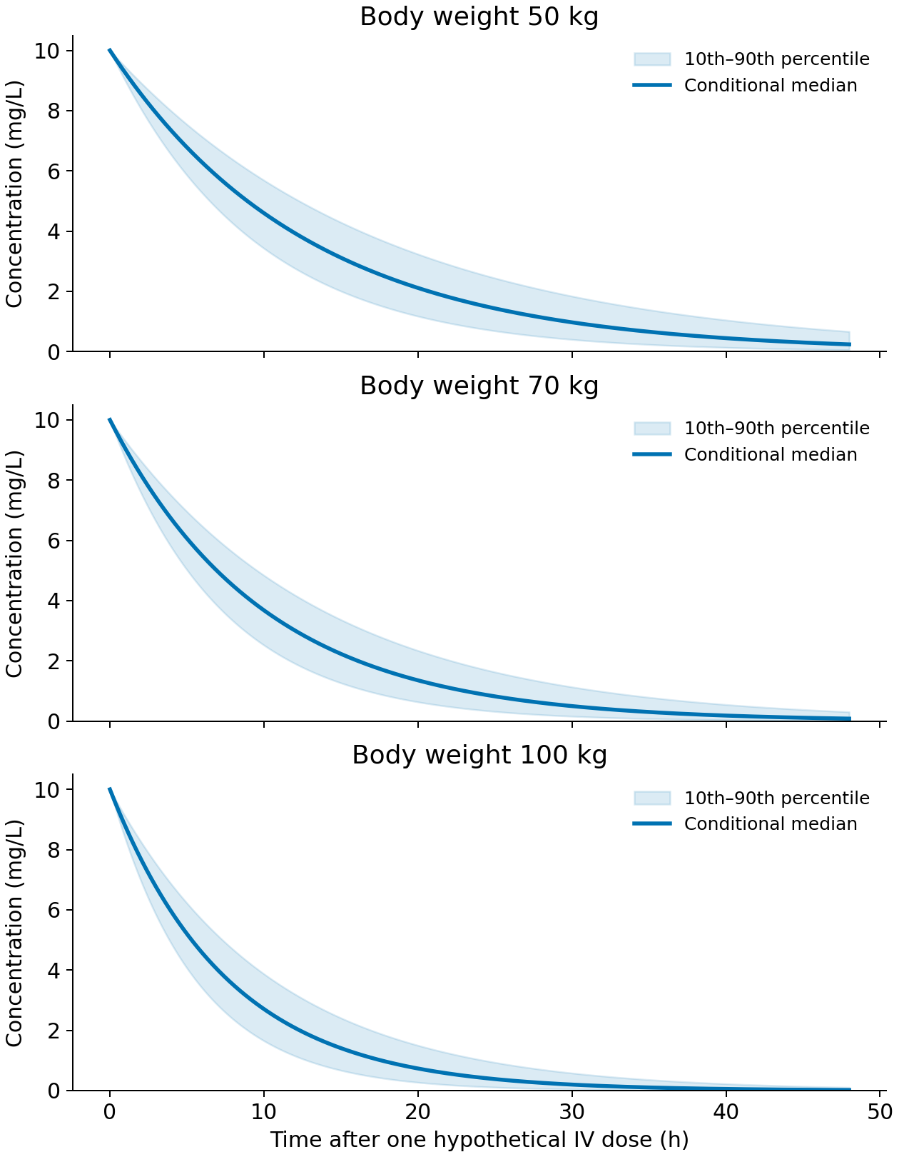
Figure 3. Typical values and variability. Lines are conditional medians; bands cover the central 80%, calculated analytically from lognormal clearance. They are not parameter confidence intervals or an observation-based VPC. Residual error, weight-dependent volume and parameter uncertainty are omitted. No actual patients or drug-specific weight adjustment are represented.
Table 5. Conditional concentrations in the illustrative distribution
| Fixed weight | Typical CL, L/h | Median concentration at 24 h, mg/L | 10th–90th percentiles, mg/L |
|---|---|---|---|
| 50 kg | 0.777 | 1.549 | 0.766–2.583 |
| 70 kg | 1.000 | 0.907 | 0.366–1.752 |
| 100 kg | 1.307 | 0.435 | 0.133–1.027 |
Outputs are population_demo.py and results/population-summary.csv. Conditional distributions overlap despite different typical values. One typical curve misses that variability; overlap alone also does not make a covariate unimportant.
Evaluating results
Model evaluation combines multiple diagnostics, rather than one attractive plot or objective-function improvement (4).
Table 6. Interpretation of population-model outputs
| Output | Evaluation focus | Misinterpretation |
|---|---|---|
| Typical parameters and uncertainty | Identification, correlations and instability | A typical value applies to everyone |
| Covariate-related exposure change | Magnitude, uncertainty and observed covariate range | Association alone determines dose changes |
| Residuals and predictions versus observations | Systematic discrepancies by time, concentration and group | Individual fit guarantees population prediction |
| Visual predictive check, VPC | Compare observed distributions with simulations reproducing observation/dose design | Any band of simulated curves is a VPC |
| Individual estimates and shrinkage | Pull toward the covariate-conditional typical value, η=0, when individual information is weak | Individual estimates are error-free observations |
High shrinkage can distort diagnostics and correlations using individual estimates. Population prediction and simulation-based checks also matter when individual information is weak. More participants or timepoints do not always provide the same improvement.
Decisions and limits
PopPK informs exposure distributions and changes by regimen or patient background. Dose decisions additionally need efficacy, safety and acceptable exposure ranges. Extrapolation to unmeasured populations or covariate ranges requires separate consideration (5). Identifying high exposure, explaining it and deciding a dose change are distinct steps.
PBPK: physiological determinants of concentration
Purpose and data
PBPK combines drug and physiological properties to examine unmeasured conditions. Physicochemical properties, binding, metabolism and transport experiments connect to organ sizes, flow, enzyme abundance and available clinical PK.
Table 7. PBPK information layers
| Layer | Example data | Evaluation focus |
|---|---|---|
| Drug | Solubility, permeability, unbound fraction, metabolism/transport rates | Experimental conditions and in vitro–in vivo scaling |
| Physiology | Organ volumes, flows, enzymes/transporters and age distributions | Population relevance, correlations and disease effects |
| Measured PK | Dose-, route- and interaction-specific concentrations | Separate construction/calibration from verification |
Physiological mass balance
PBPK represents movement and elimination using physiology. Naming a conventional peripheral compartment after an organ does not by itself establish physiological modeling.
For a non-eliminating tissue with perfusion-limited distribution, a simplified balance is
\[ V_T\frac{dC_T}{dt}=Q_T\left(C_A-\frac{C_T}{K_{p,T}}\right) \]
\(V_T\) is tissue volume, \(Q_T\) flow, \(C_A\) arterial blood concentration, \(C_T\) tissue concentration and \(K_{p,T}\) the tissue:blood partition coefficient. The same concentration basis is used, with venous concentration approximated by \(C_T/K_{p,T}\). Eliminating organs, permeability limitation or separately represented blood-cell partitioning need additional terms or structures.
Separating drug from system properties supports questions about enzyme inhibition, pediatric physiology or organ dysfunction, provided the relevant mechanisms and information are present. FDA reporting guidance describes combining physiological, population and drug properties; replacing clinical PK data is judged case by case for intended use and result quality (6). A PBPK label alone does not guarantee extrapolation.
Not every organ must be represented in detail. Models can retain only relevant components, and unknown parameters can be estimated. PBPK is not invariably fixed entirely by literature, nor conventional PK entirely by clinical data (1, 7). Tissue concentrations also do not automatically determine efficacy or safety; connecting PD or disease models leads to PBPK/PD or integration with QSP.
Interpretation and intended use
Relevant outputs include profiles, AUC, Cmax, interaction ratios and population distributions. Inhibition extrapolation requires appropriate metabolic and inhibitory mechanisms and verification conditions informative for the target application. One fold-error threshold should not be applied mechanically to every use.
Platform performance, individual drug-model performance and applicability to the current use differ. Matching blood concentrations does not uniquely identify unmeasured tissue exposure or pathway contributions. Sensitivity and uncertainty in influential unknowns require examination (7).
QSP: connecting drug action and biological systems
Purpose and data
QSP considers why similar exposure yields different responses, combination mechanisms and disease influences on drug action. Relevant binding, signaling, cell-function, animal/human disease, PK, biomarker and clinical information are combined as needed.
Linking systems, species and measurement scales requires recording units, conditions and transformations. Sources sharing participants or experiments are not independent evidence. Many data types do not guarantee precise parameters.
Pharmacology and disease mechanisms
QSP quantitatively integrates pharmacology with interactions among pathways, cells, tissues and disease. It can connect target engagement to signaling, cell-state changes and disease response.
A September 2026 review presents mechanism-based biology and quantitative pharmacology for dose/regimen, combination and biomarker-stratification questions (8). QSP is not one fixed equation or estimation algorithm.
Table 8. Conceptual relationships in a T-cell-mediated drug model
| Relationship | Analytical role | Relevant evidence |
|---|---|---|
| Exposure and target binding | Entry to pharmacological action | Concentrations, binding and target abundance |
| Immune–tumor-cell interaction | Antitumor response | Cell counts, activation and killing over time |
| Activation, cytokines and regulation | Amplification and control | Timed biomarkers and background differences |
| Tumor growth and treatment | Observable disease change | Pretreatment and on-treatment dynamics |
This is a conceptual example, not a validated drug-specific model or mandatory mechanism list. Additional mechanisms increase parameter, data-consistency and identifiability demands.
Definitions vary, with overlap with PK/PD and PBPK (9). No fixed number of molecular variables defines QSP. Explicit interactions and testable hypotheses are more useful. Modeling can propose experiments, with observations revising mechanisms and parameters.
Varying parameters does not automatically create a real patient population. Relevant questions concern calibration observations, covariate correlations and independent checks.
Interpretation and limits
Calibration adjusts parameters or virtual populations to data; agreement on those data differs from independent validation. Removing mechanisms, varying plausible parameters or structures, and examining unobserved responses can reveal whether decisions are stable.
Reading virtual-population fractions as clinical response rates requires evidence-based composition and weights. More virtual patients do not repair model error. An elranatamab example links virtual populations to clinical response, but its settings and evaluation do not transfer automatically to another drug (10).
QSP informs hypotheses and unmeasured-condition contrasts and helps focus data collection. Clinical predictions used for decisions need intended-use validation. Biological detail does not equal predictive accuracy.
Structure, variability and estimation are separate axes
PopPK concerns population PK, variability and covariates. NLME combines population parameters with individual random effects in a statistical framework. Representing concentrations/responses and representing/estimating variability are related but distinct questions (11, 5).
A one-compartment PK/PD model can use NLME. PBPK parameters can have population distributions, and QSP can be calibrated to population data. Simulating a virtual population is not equivalent to fitting mixed effects to individual observations.
Pharmacometrics is the broader quantitative study of drugs, disease and variability to inform decisions, not a synonym for NLME or PopPK. Terminology varies across fields and organizations. Recent work connects QSP and pharmacometrics rather than treating names as fixed boundaries (12).
Discussion
Model combinations should follow the decision question.
Table 9. Illustrative starting points for different questions
| Question | Possible starting approach | Evidence to examine |
|---|---|---|
| Explain observed-dose/population concentrations and variability | PopPK, linked to PK/PD if needed | Sampling, covariates, variability and diagnostics |
| Explain response delays or compare intervals | Mechanism-based PK/PD | Response time series, delay hypotheses and intended-use validation |
| Predict unmeasured interactions or physiology | PBPK with relevant mechanisms | Enzymes/transporters, physiology and nearby empirical conditions |
| Examine multiple pathways, cells or combinations | QSP linked to PK/PBPK exposure | Mechanistic evidence, calibration, sensitivity and independent verification |
| Disease changes both exposure and response | Linked PK/PD/disease model | Feedback, confounding and unobserved states |
These are not unique choices. PopPK can inform observed interactions, and QSP can compare intervals. The appropriate model can change with the question for the same drug.
Intended-use verification
ICH M15, adopted at Step 4 on January 29, 2026, names population PK/PD, PBPK and QSP among MIDD methods used individually or together (13). Regional implementation requires separate checking. Its shared principle is a defined question, role and scope, with evaluation proportionate to decision impact and consequences of error.
An April 2026 ISoP QSP SIG preprint proposes transparent, use-dependent reporting (14); it is not new official regulatory guidance. Model names alone do not establish credibility.
Conclusion
The synthetic example connects one concentration trajectory to different responses. More physiological or pathway detail alone does not make a response correct. Observations supporting each structure, its assumptions and its use determine prediction limits more directly than whether it is called PK/PD, PBPK or QSP.
Data and code availability
python model_demo.py generates figures/CSVs, and python -m unittest test_demo.py -q checks them. Python, NumPy, SciPy and Matplotlib are used without randomness or patient data. This illustrates basic PK/PD connections; it neither constructs, estimates nor validates actual-drug PBPK/QSP models and does not support dosing decisions.
Figure 3 and its table use python population_demo.py. All checks run with python -m unittest discover -p 'test_*.py' -q. Population distributions are assumed, without fitting NLME to individual observations.
Download figures and calculation code
References
- Jusko WJ. Moving from Basic Toward Systems Pharmacodynamic Models. Journal of Pharmaceutical Sciences. 2013;102(9):2930–2940. doi:10.1002/jps.23590.
- Upton RN, Mould DR. Basic Concepts in Population Modeling, Simulation, and Model-Based Drug Development: Part 3—Introduction to Pharmacodynamic Modeling Methods. CPT: Pharmacometrics & Systems Pharmacology. 2014;3(1):e88. doi:10.1038/psp.2013.71.
- Mould DR, Upton RN. Basic Concepts in Population Modeling, Simulation, and Model-Based Drug Development—Part 2: Introduction to Pharmacokinetic Modeling Methods. CPT: Pharmacometrics & Systems Pharmacology. 2013;2(4):e38. doi:10.1038/psp.2013.14.
- Nguyen THT, Mouksassi MS, Holford N, Al‐Huniti N, Freedman I, Hooker AC, et al. Model Evaluation of Continuous Data Pharmacometric Models: Metrics and Graphics. CPT: Pharmacometrics & Systems Pharmacology. 2017;6(2):87–109. doi:10.1002/psp4.12161.
- US Food and Drug Administration. Population Pharmacokinetics: Guidance for Industry. 2022 Feb. Final guidance.
- US Food and Drug Administration. Physiologically Based Pharmacokinetic Analyses: Format and Content. Guidance for Industry. 2018 Sep. Final guidance.
- Shebley M, Sandhu P, Emami Riedmaier A, Jamei M, Narayanan R, Patel A, et al. Physiologically Based Pharmacokinetic Model Qualification and Reporting Procedures for Regulatory Submissions: A Consortium Perspective. Clinical Pharmacology & Therapeutics. 2018;104(1):88–110. doi:10.1002/cpt.1013.
- Wang W, Ratushny AV, Chang S, Cheng Y, Gong JQX, Gulati A, et al. Quantitative Systems Pharmacology (QSP): Bridging Biology and Mechanism with Clinical Drug Development Decisions. The Journal of Clinical Pharmacology. 2026;66(9):e70289. doi:10.1002/jcph.70289.
- Bradshaw EL, Spilker ME, Zang R, Bansal L, He H, Jones RDO, et al. Applications of Quantitative Systems Pharmacology in Model-Informed Drug Discovery: Perspective on Impact and Opportunities. CPT: Pharmacometrics & Systems Pharmacology. 2019;8(11):777–791. doi:10.1002/psp4.12463.
- Poels KE, Elmeliegy M, Hibma J, Wang D, Musante CJ, Shtylla B. Leveraging quantitative systems pharmacology modeling for elranatamab regimen optimization in relapsed or refractory multiple myeloma. npj Systems Biology and Applications. 2025;11(1):102. doi:10.1038/s41540-025-00585-z.
- Mould DR, Upton RN. Basic Concepts in Population Modeling, Simulation, and Model-Based Drug Development. CPT: Pharmacometrics & Systems Pharmacology. 2012;1(9):e6. doi:10.1038/psp.2012.4.
- Kapitanov GI, Earp JC, Gadkar K, Jin JY, Joshi A, Kondic AG, et al. Bridging the Gap: Integrating Quantitative Systems Pharmacology and Pharmacometrics in Drug Development. Clinical Pharmacology & Therapeutics. 2026;119(4):830–833. doi:10.1002/cpt.70191.
- International Council for Harmonisation. General Principles for Model-Informed Drug Development: M15. Step 4 final guideline. 2026 Jan 29. Final guideline.
- Zaph S, Shtylla B, Chang S, Cheng Y, Gong JQX, Gulati A, et al. Best Practices on QSP Model Reporting for Regulatory Use: perspectives from ISoP QSP SIG Working Group. arXiv [Preprint]. 2026 Apr 9;2604.07811v1. Preprint.