From public T-cell engager evidence to the next experiment
Public PopPK and efficacy reconstruction, Bayesian CRS sensitivity, and hypothetical measurement value and sampling design.
Key findings
- Using the published tarlatamab PopPK and Emax models in 5,000 virtual subjects, initial exposure matched label summaries, but steady-state troughs did not fully agree.
- Bayesian models of three aggregate CRS windows fitted the data, but the exposure-history timescale depended on the prior, so no optimal step-up among 14 schedules could be chosen.
- Matching dose intensity preserved average exposure but changed peaks and troughs, and early-only sampling did not stabilize CL; the framework specifies which measurements could change a decision, not a validated regimen.
On this page
- 日本語要約
- Abstract
- 1. Regimen design is more than choosing a target dose
- 2. Question of interest and context of use
- 3. Evidence, reconstructions, and assumptions
- 4. Reference-covariate two-compartment PopPK
- 5. Formal efficacy E–R
- 6. What the CRS summaries motivate
- 7. A generalized Bayesian history model
- 8. Fit is easier than identification
- 9. Step-up scenarios and their uncertainty
- 10. Priming adequacy is a missing measurement
- 11. Maintenance exposure and a drug-specific margin
- 12. A dimensionless molecule feasibility map
- 13. Decision value of the next measurement
- 14. PK and cytokine sampling designs
- 15. Experiment → parameter → decision
- 16. Updating for a molecule with new data
- 17. Validation and boundaries
- 18. Reproduce the analysis
- 19. Measurements needed next
- References
日本語要約
T-cell engagerの投与設計では、有効性に必要な曝露、初期の免疫刺激、投与履歴、維持期の濃度を分けて考える必要がある。本解析はタルラタマブの公開2コンパートメントPopPKと正式Emaxモデルを再計算し、CRS集計に曝露履歴を加えたBayesian探索モデルを適用した。5,000人の仮想被験者と14条件のstep-upを比較したが、CRSの絶対値と履歴半減期は仮定に依存し、最適レジメンは決められなかった。別に、仮想薬剤の成立条件、実験の近似情報価値、採血設計を計算した。平均曝露を保存してもピークとトラフは変わり、初期採血を増やすだけではCLの推定が安定しない。これらは公開情報の再現と仮定したシナリオを分け、次に測定すべきものを具体化する方法である。患者のリスク予測、新しい薬剤の用量提案、実験投資の確定順位には使用しない。
Abstract
Public clinical pharmacology evidence can inform regimen questions before molecule-specific data become available, but its evidential limits must remain visible. We reconstructed a reference-covariate two-compartment tarlatamab model, propagated published interindividual variability in 5,000 virtual subjects, and used published ORR and DCR Emax parameters. Nine generalized Bayesian model and sensitivity conditions examined three overlapping aggregate CRS windows. Fourteen step-up schedules were compared, followed by steady-state maintenance simulations. A separate, explicitly hypothetical model explored dimensionless molecule feasibility, approximate decision value of measurements, and PK/cytokine sampling designs. Initial mean exposures were reasonably close to label summaries, whereas steady-state trough agreement remained incomplete. Exposure-history and administration-category models both described the three CRS summaries; the history timescale remained prior-sensitive despite satisfactory sampling diagnostics. Equal dose intensity preserved average exposure while changing peaks and troughs. In hypothetical decision scenarios, priming measurements had substantial value, but rankings depended on assumed utility and measurement models. Local information calculations showed weak CL identification from early-only sampling. These results support a reproducible route from evidence to testable measurement requirements, rather than identification of a clinically optimal schedule. No individual clinical data were used, and neither the CRS extrapolations nor hypothetical assay rankings are validated clinical predictions.
1. Regimen design is more than choosing a target dose
A schedule must address efficacy exposure, acute immune activation, and pharmacologic coverage over time. A small initial dose can reduce an acute stimulus but may also fail to produce a sufficient priming response. A longer maintenance interval can preserve average exposure while changing its waveform.
The preceding PK analysis separated these questions. Here, we extend the analysis to a history model and to the decision value of additional measurements. These extensions deliberately add assumptions. Their purpose is to expose which assumptions drive decisions, not to make sparse public data appear more informative.
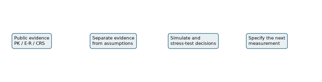
Figure 1. Analytical workflow. Clinical reconstruction and hypothetical decision scenarios are separate evidence streams; a fitted clinical posterior is not automatically transferred to a new molecule.
2. Question of interest and context of use
QoI: Which parts of a T-cell engager regimen comparison are supported by public evidence, which depend on assumptions about exposure history and priming, and which measurements could resolve those assumptions?
CoU: Public-data reconstruction, methodological scenario comparison, and preparation of measurement requirements. The framework does not choose a patient dose, a first-in-human starting dose, or a clinical step-up/maintenance schedule. The hypothetical scores below are not clinical success or CRS probabilities.
This framing is consistent with the emphasis on efficacy, safety, and tolerability in FDA Project Optimus and its Oncology Dosing Tool Kit. ICH M15, finalized by FDA in June 2026, provides a context for defining model use and supporting evidence. None of these resources endorses this particular simulation.
3. Evidence, reconstructions, and assumptions
| Evidence | Use | Limits |
|---|---|---|
| FDA tarlatamab review, Tables 66–67 [1] | Structural PK and IIV | Reference parameters do not recover the trial covariate distribution |
| Tarlatamab PopPK [2] and label Table 17 [3] | Model context and exposure benchmarks | Benchmarks are model-derived means, not raw observations |
| Formal tarlatamab E–R, Supplementary Table S1 [4] | ORR/DCR Emax | Patient-level dosing records and outcomes unavailable |
| DeLLphi-301 AE-management Figure 2 [5] | 54/133, 39/133, 10/133 all-grade CRS | Repeated subjects; windows are 7, 7, and 14 days |
| Epcoritamab RTTE analysis [6] | Structural comparison | Grade ≥2 CRS, CD20 disease, SC administration; no numeric parameter transfer |
| Teclistamab modeling [7] | Example of a pharmacologic exposure margin | Different molecule, endpoint and responder population |
| Mosunetuzumab step-up analysis [8] | Example of drug-specific PK/RO/CRS linkage | Anti-CD20 competition and exposure metrics are not interchangeable |
No individual participant-level clinical data were used. We label published counts observed, source parameter estimates published model-derived, our calculations reconstructed, and untested regimens/hypothetical molecules exploratory. Sources were checked on 2026-10-03. Public source material is retained for audit but excluded from the downloadable package; source URLs are included.
4. Reference-covariate two-compartment PopPK
For amounts in mg, volumes in L, and time in days:
\[ \dot A_c=R_{in}-(CL+Q)A_c/V_c+QA_p/V_p,\qquad \dot A_p=QA_c/V_c-QA_p/V_p,\qquad C=A_c/V_c. \]
The infusion duration is 1 hour. FDA values are CL=0.649 L/day, Vc=3.44 L, Vp=5.06 L, and Q=1.11 L/day [1]. The reference is 73 kg, White, binding ADA-negative. CL and Vc are lognormally distributed with η SDs 0.437 and 0.387 and correlation 0.535. These are SD/correlation values, not CV values requiring a second transformation. Residual error is not added to latent exposure.
The analytical infusion solution was checked against a matrix exponential, numerical AUC integration, and repeated-dose accumulation. The reference terminal half-life is approximately 11.2 days. All 5,000 subjects retain reference covariates, and the same subject is used across schedules. This reproduces the full two-compartment structure, not all covariate distributions or actual trial dosing histories.
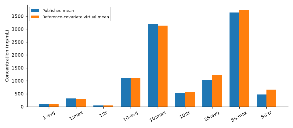
Figure 2. Concentrations in ng/mL. 1 and 10 denote the first 1 mg and first 10 mg intervals; SS denotes steady 10 mg Q2W. Published means and virtual means refer to different populations. No interval is implied for the published point summaries.
| Period | Metric | Published mean | Virtual mean | Difference |
|---|---|---|---|---|
| First 1 mg | Cavg | 106 | 106.2 | +0.2% |
| First 1 mg | Cmax | 314 | 308.1 | −1.9% |
| First 1 mg | Ctrough | 49 | 51.6 | +5.4% |
| First 10 mg | Cavg | 1,100 | 1,103.4 | +0.3% |
| First 10 mg | Cmax | 3,190 | 3,132.8 | −1.8% |
| First 10 mg | Ctrough | 517 | 550.0 | +6.4% |
| Steady Q2W | Cavg | 1,040 | 1,211.7 | +16.5% |
| Steady Q2W | Cmax | 3,640 | 3,742.4 | +2.8% |
| Steady Q2W | Ctrough | 472 | 662.5 | +40.4% |
The steady trough discrepancy prevents qualification as a complete reproduction of label population exposure. At η=0, the corresponding discrepancy is about +16%; adding IIV changes the mean. Matching a typical value to a population mean would conceal this distinction. Relative within-model comparisons remain computable, but absolute threshold claims are not justified by this benchmark.
The source reports weight, ADA and race effects [1,2]. A separate covariate bracket uses the reported proportional coefficients with both linear and exponential weight forms, because the exact weight functional form was not independently confirmed. These calculations are labeled assumptions and are not called a reproduction of the full covariate model.
5. Formal efficacy E–R
The published model is
\[ p(E)=E_{max}E/(EC_{50}+E),\qquad E=C_{avg,\mathrm{first\ cycle}}. \]
Supplementary Table S1 gives ORR Emax=0.339 and EC50=57.4 ng/mL (95% CI 22.5–146), and DCR Emax=0.650 and EC50=49.4 ng/mL (20.9–117) [4]. These formal estimates are used throughout the reconstructed efficacy calculations.
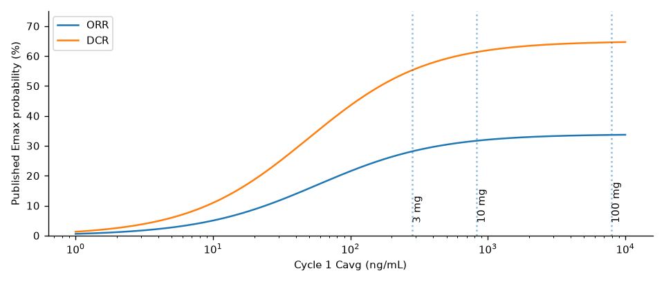
Figure 3. Published Emax parameters; vertical lines are reconstructed Cycle-1 median Cavg for a common 1 mg→target→target schedule. They are not observed cohort exposure medians. Curves show point estimates, not prediction bands.
At reconstructed medians for 3/10/100 mg, ORR is 28.2/31.7/33.7%, compared with the original paper's reported 26.2/31.4/33.6%. DCR is 55.3/61.4/64.6%, compared with 52.0/60.8/64.5% [4]. The common schedule and reference-covariate population do not reconstruct the original pooled actual dosing records. We therefore reproduce the function, but do not claim exact reproduction of all cohort predictions.
An E90 of 9×EC50 means 90% of the model maximum, not 90% response. Neither this Cycle-1 average-exposure relation nor its plateau supplies a maintenance trough threshold. A response model transferred to a new schedule is an exploratory calculation, not demonstrated efficacy equivalence. One-at-a-time EC50 endpoint sensitivity for every schedule is supplied in results/efficacy-sensitivity.csv; it does not propagate a joint Emax–EC50 posterior.
6. What the CRS summaries motivate
The observed all-grade proportions are 40.6%, 29.3% and 7.5% across D1–7, D8–14 and D15–28 [5]. Reference-model peaks increase across the corresponding administrations.
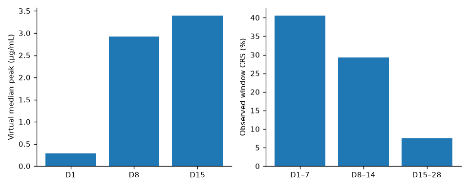
Figure 4. Left: virtual median peaks in µg/mL. Right: observed aggregate window proportions. These are not patient-matched exposure–event pairs. The last window is twice as long as the first two.
A shared monotone-increasing exposure-only model cannot describe this particular ordering under its assumptions. An unconstrained exposure-only model can instead learn a negative slope. Neither result proves biological adaptation: prophylaxis, changing disease burden, selection, timing and repeated events remain possible explanations. Administration-category terms provide another descriptive solution.
Epcoritamab RTTE modeling in 600 subjects used stimulation and inhibition components and included prophylaxis and prior CAR-T effects [6]. It supports considering exposure history, but its Grade ≥2 hazard parameters cannot be inserted into an all-grade tarlatamab probability model. No quantitative epcoritamab prior was borrowed here.
7. A generalized Bayesian history model
For normalized peak \(x_{ik}=C_{max,ik}/(1\,\mu g/mL)\):
\[ H_{ik}=\sum_{m<k}\frac{x_{im}}{r+x_{im}} \exp\{-\ln(2)(t_k-t_m)/T_H\}, \qquad p_{ik}=\operatorname{logit}^{-1}(\alpha+\beta\log x_{ik}-\gamma H_{ik}). \]
We average p over a fixed 256-subject reference-covariate integration sample. H is a phenomenological exposure-history state, not established immune tolerance. Its effect may absorb unmeasured differences between periods.
| Parameter | Baseline prior | Interpretation |
|---|---|---|
| α | Normal(logit(0.4), 1.5²) | Exploratory baseline log-odds |
| log β | Normal(log(0.43), 0.7²) | Assumed positive acute slope; not an external estimate |
| log γ | Normal(log(2), 0.7²) | Assumed attenuation strength |
| log TH | Normal(log(20), 0.8²) | Assumed history timescale, days |
| log r | Normal(log(0.1), 1.5²) | Assumed dimensionless saturation scale |
Because the same patients occur in different windows, the product of three binomial likelihoods is not a recovered joint likelihood. We instead use an explicitly exploratory power composite likelihood:
\[ q(\theta\mid y)\propto p(\theta) \left\{\prod_{k=1}^3\mathrm{Binomial}(y_k;133,\bar p_k(\theta))\right\}^{w},\quad w=0.5. \]
Sensitivity uses w=0.25 and 1. Down-weighting does not solve the unknown dependence; it only exposes sensitivity to an assumed information scale. The resulting intervals are generalized-posterior intervals, not calibrated patient-risk confidence intervals.
We fit positive-slope exposure-only, unconstrained exposure-only, administration-category and continuous-history models, plus wider-prior and fast/slow-history conditions. Each uses four NUTS chains, 1,500 tuning and 1,200 retained draws per chain. Across nine fits, maximum R-hat is below 1.008, minimum bulk ESS exceeds 816, and there are zero divergences. These diagnostics assess sampling, not model identification.
8. Fit is easier than identification
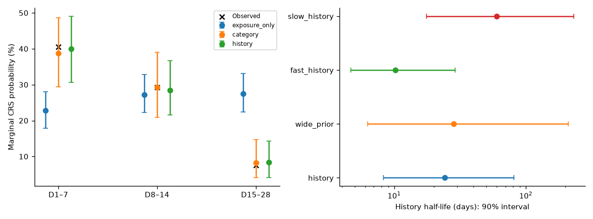
Figure 5. Left: generalized-posterior medians and 90% intervals for each window; crosses are observed proportions. Right: history-timescale intervals under different priors. These are fitted marginal probabilities, not joint longitudinal validation or out-of-sample checks.
| Window | Observed | Positive exposure-only | Category | History |
|---|---|---|---|---|
| D1–7 | 40.6% | 22.8% | 38.8% | 39.9% |
| D8–14 | 29.3% | 27.2% | 29.3% | 28.5% |
| D15–28 | 7.5% | 27.5% | 8.2% | 8.4% |
Marginal replicated-count checks are saved in results/crs-ppc.csv. Each window is simulated conditional on its fitted probability; these checks do not recover the unknown joint dependence between windows. Both category and history models can describe these summaries. This does not select the history model as a unique mechanism. Baseline history-model medians (90% intervals) are β=0.334 (0.121–0.751), γ=2.38 (1.42–4.42), TH=24.1 days (8.3–81.0), and r=0.088 (0.0087–0.549).
With prior centers of 5 versus 60 days, TH intervals shift to approximately 4.7–29.1 versus 17.6–231.5 days. A plausible fit to three summaries therefore does not establish a 20-day adaptation constant.
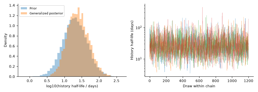
Diagnostic figure. Prior/posterior overlap and chain behavior. Broad intervals and prior sensitivity remain despite converged traces. Results are stored in chain-ordered NPZ files and diagnostic tables.
9. Step-up scenarios and their uncertainty
Fourteen prefixes are tested at 7-day spacing. After the first 10 mg target administration, another 10 mg is given 7 days later, then every 14 days. Thus the 1→10 prefix reproduces D1/D8/D15; direct 10 uses D1/D8/D22. This rule is a defined counterfactual geometry, not an approved direct-dose regimen. Cycle 1 is days 0–28 for every comparison.
| Prefix | Target day | Transferred DCR median | Maximum marginal CRS median |
|---|---|---|---|
| Direct 10 | 0 | 62.3% | 59.0% |
| 0.1→10 | 7 | 61.2% | 46.8% |
| 0.5→10 | 7 | 61.3% | 38.2% |
| 1→10 | 7 | 61.4% | 40.7% |
| 3→10 | 7 | 61.7% | 49.5% |
| 0.3→1→10 | 14 | 60.6% | 31.7% |
| 0.3→1→3→10 | 21 | 58.2% | 31.5% |
CRS summaries combine 400 posterior draws with 250 virtual subjects; sensitivity comparisons use 200 draws and 100 subjects. Marginal p intervals for every administration, full exposure distributions, and sensitivity results are supplied in the result tables. Maximum marginal probability is not the probability of any CRS over the complete schedule; event dependence prevents that calculation. The extension associates one peak with each observed window without fitting event-time hazards. Its administration outputs are not risks over a common follow-up duration: the 7/14-day observation-window difference cannot be corrected from these summaries.
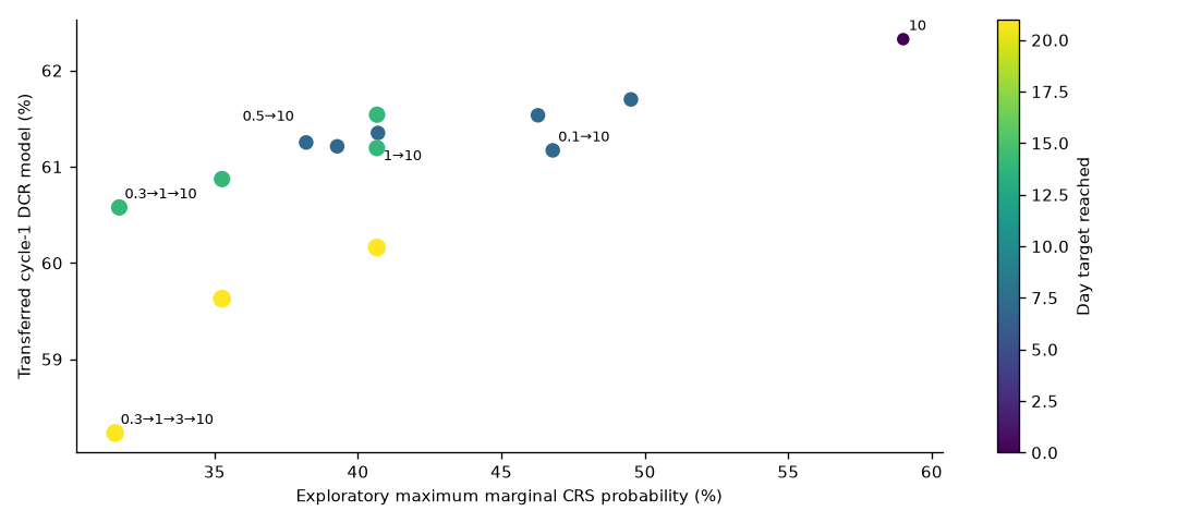
Figure 6. Points are medians, color is target day and size reflects step count. Labels are limited for legibility; all 14 schedules and intervals are available in CSV. The axes are transferred model outputs, not clinically validated outcomes. The Pareto analysis includes DCR, maximum marginal CRS, target day and administration count; being non-dominated is not a clinical recommendation.
For direct 10, the sensitivity run gives approximately 59.6% (47.1–80.7%) in the baseline condition. This interval is conditional on the stated priors, likelihood treatment, integration population and schedule geometry; it is not an externally validated risk estimate.
Very small priming doses do not necessarily minimize predicted CRS: a 0.1 mg prefix leaves less history attenuation before the target dose in this model. Conversely, this model cannot establish how much priming is sufficient. Changes in absolute CRS values or rankings under assumptions should be treated as fragility, not optimization evidence.
10. Priming adequacy is a missing measurement
A candidate bounded priming response is
\[ P(E)=E^{h_p}/(P_{50}^{h_p}+E^{h_p}). \]
This notation is a response index unless a probabilistic endpoint and observation model are specified. A useful experiment would measure initial stimulation, washout, and rechallenge under a fixed target-cell/T-cell configuration. It must assess both the reduction in the second cytokine response and retained cytotoxic function. A reduction in cytokines caused by cell loss or impaired killing is not adequate priming.
The data needed include dose/concentration, exposure duration, interchallenge interval, viability, CD69/CD25, cytokines and TDCC. Donor and target-density variation should be paired across conditions. Safety-only optimization is incomplete, but adding an arbitrary priming cutoff does not make it clinically complete.
11. Maintenance exposure and a drug-specific margin
The population is simulated at steady state under six conditions. For each subject, metrics are divided by their own 10 mg Q2W value.
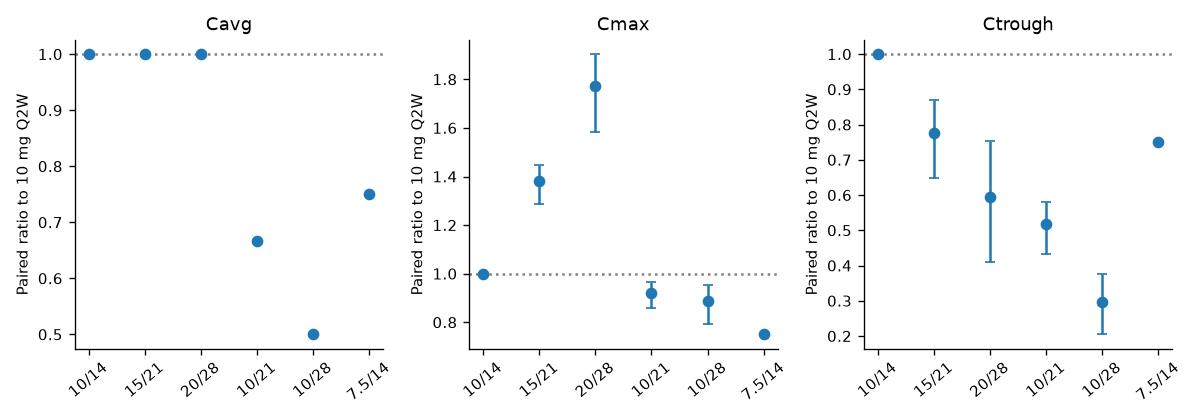
Figure 7. Median and 5–95% IIV ranges. Equal-dose-intensity schedules preserve Cavg, but 15 mg Q3W raises peaks by approximately 38% and lowers troughs by approximately 22%; 20 mg Q4W raises peaks by approximately 78% and lowers troughs by approximately 40%. These are PK comparisons, not efficacy-equivalence claims.
Teclistamab supplies an example of a different evidence chain: median estimated troughs of 20.4, 14.4 and 11.7 µg/mL were compared with an ex-vivo cytotoxicity EC90,max of 6.039 µg/mL [7]. The resulting calculated margins are 3.38, 2.38 and 1.94. The threshold came from five patient bone-marrow samples, and the switching analysis concerned responders. It is neither a universal TCE threshold nor a sufficient condition for every patient. No such validated tarlatamab maintenance margin is introduced here.
12. A dimensionless molecule feasibility map
We separately define a hypothetical one-compartment bolus model. Normalized TDCC E90 is 1; functional TI is cytokine E50/TDCC E90. Its units are not convertible to tarlatamab mg. The model has no fitted clinical CRS likelihood.
For dose D, volume scale V, interval τ and elimination k=ln2/half-life:
\[ C_{max,ss}=\frac{D/V}{1-e^{-k\tau}},\quad C_{trough,ss}=C_{max,ss}e^{-k\tau},\quad C_{avg,ss}=\frac{D}{Vk\tau}. \]
We use 160 grid actions: normalized doses 1/2/4/8; intervals 3/7/14/21/28 days; priming fractions 0.03/0.1/0.3/0.5; and one/two priming administrations separated by 7 days. Hypothetical immune stimulation is S(C)=C/(cytokine E50+C), attenuated at rechallenge by exp(−γH). P50=0.3, γ=2 and history half-life=10 days are assumed. Peak residual drug and each previous priming administration are included; the worst early stimulation score is retained.
Across TI=1–100 and half-life=1–21 days, each condition uses 500 virtual subjects with log-SDs 0.35 for half-life and 0.30 for volume. A grid action is called feasible only if at least 90% have trough/E90>1, at least 80% have early stimulation below the stated limit, and at least 80% meet the priming-response limit. These are illustrative constraints.
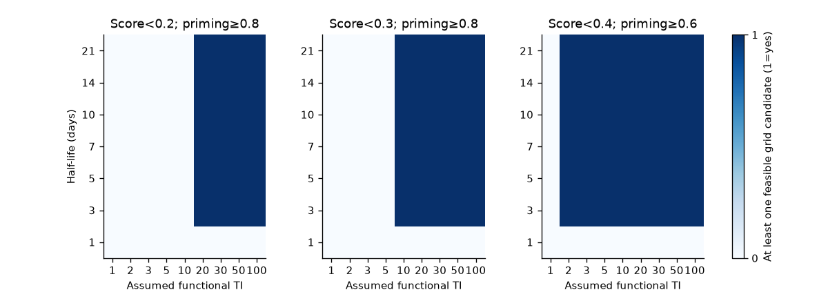
Figure 8. Binary existence of at least one feasible candidate in a finite grid. Blue does not indicate a probability of clinical success. White does not establish that no feasible schedule exists outside the grid. Broader TI and longer half-life can help in this structure, but dose grid, variability, priming and thresholds materially affect the boundary.
13. Decision value of the next measurement
The purpose of an assay is to change or stabilize a defined decision. We therefore evaluate expected utility, rather than labeling a reduction in parameter variance as value of information.
For normalized efficacy score E, stimulation score S, priming index P, maintenance margin M, number of priming administrations N and interval τ:
\[ U=E-w_S S-w_P\max(0.8-P,0) -w_M\frac{\max(1-M,0)}{1+\max(1-M,0)}-0.02N-0.02(7/\tau). \]
Here E=Cavg/(Cavg+E90/9), including an assumed target-density multiplier. All weights are dimensionless preferences, not health utilities. We evaluate (wS,wP,wM)=(1,1,0.3), (2,1,0.3), and (1,2,0.6).
Eight independent lognormal uncertainties are assigned to half-life, TDCC E90, cytokine E50, priming P50, history half-life, history strength, target-density factor and volume scale. Their assumed medians/log-SDs are in data/generic-assumptions.json. Independent 6,000-sample training and test draws prevent choosing and evaluating the same conditional decision on one sample.
EVPI is estimated as E[maxa U(a,θ)]−E[U(a0,θ)]. Partial information uses 12 bins of one parameter or its noisy log-measurement, selects an action in each training bin and evaluates that action out-of-sample. We report this as binned EVPPI/EVSI approximation, not exact posterior integration. Assay log-error SDs 0.15 and 0.40 are hypothetical.
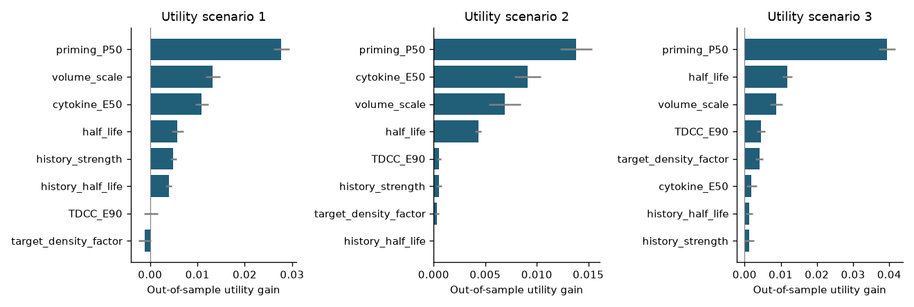
Figure 9. Test-set mean utility gain, with Monte Carlo ±1.96 SE for the fixed trained policy. These bars do not include training-policy or structural uncertainty. They are not assay-cost-adjusted investment rankings.
| Measurement, log-error SD 0.15 | Utility scenario 1 | Scenario 2 | Scenario 3 |
|---|---|---|---|
| Priming P50 | 0.0277 | 0.0138 | 0.0394 |
| Cytokine E50 | 0.0109 | 0.0091 | 0.0020 |
| PK half-life | 0.0058 | 0.0043 | 0.0118 |
| TDCC E90 | 0.0001 | 0.0005 | 0.0045 |
Priming information has value in these scenarios because priming uncertainty and inadequacy carry explicit penalties. This is a conditional result, not a universal ranking of experiments. A nearly zero or slightly negative approximate gain reflects finite-sample/binning error and an imperfect decision rule; exact information value cannot be negative when retaining the old decision remains allowed. We do not convert these gains into percentages of uncertainty reduction or financial benefit.
Tumor-growth/kill measurements are not given a numeric information-value rank: this toy utility has no fitted tumor-growth component. Assigning a value anyway would manufacture a decision model that was not analyzed.
14. PK and cytokine sampling designs
We calculate local Fisher information for log(CL,Vc,Q,Vp), with assumed independent log-concentration error SD 0.30. Concentrations follow 1→10→10 mg at days 0/7/14; the residual SD is an assumed design value, not the FDA's reported residual SD. Information is per subject and excludes BLQ, random effects, dropout and between-occasion variation. Pre-dose zero concentrations contribute no log-information.
| Design | Postdose sampling times | Reference SE log(CL) |
|---|---|---|
| Sparse early | 1/6/24 h, day 7 | 85.16 |
| Intermediate early | 1/4/8/24/48 h, day 7 | 12.49 |
| Dense early | 1/2/4/8/24/48/72 h, day 7 | 5.39 |
| Sparse + late | Sparse plus days 14 and 28 | 0.324 |
| Dense + late | Dense plus days 14 and 28 | 0.278 |
Day-7 and day-14 samples are before their infusions. Extremely large early-design values indicate ill-conditioning; the local approximation is not a usable precision forecast in that range. Fixing Q and Vp would give an artificially easier problem. CL multipliers 0.5 and 3.33 are also tested; these alter terminal half-life through the two-compartment system and are not literal half-life multipliers.
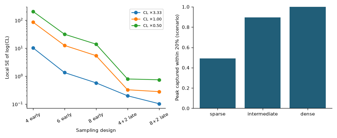
Figure 10. Left: log(CL) SE under three CL conditions; early sample density alone is insufficient. Right: peak capture in an assumed cytokine scenario, not observed clinical kinetics.
For cytokines, we assume peak time uniformly distributed from 2–12 h and response exp{−0.5[log(t/tpeak)/0.6]²}, with no measurement error. Capturing at least 80% of the true peak occurs in 49.2% of simulations for 0/6/24 h, 89.6% for 0/2/6/12/24 h and 100% for 0/2/4/6/12/24 h. The last value follows the smooth assumed peak shapes and timing range; it does not guarantee clinical peak capture. Kinetic and assay noise sensitivity is required before using a real sampling recommendation.
15. Experiment → parameter → decision
| Experiment | Information | Decision it can support |
|---|---|---|
| TDCC concentration-response, multiple donors | E50/E90, Hill shape | Target-exposure assumptions |
| Target-density panel | Potency shift and donor variability | Coverage robustness across disease states |
| Cytokine response alongside TDCC | Separation of killing and stimulation | Functional TI hypotheses |
| Priming/washout/rechallenge | P50, retained killing, history/time dependence | Step fraction and interval hypotheses |
| Mouse PK, concentrations and repeated-dose tumor volumes | PK and growth/kill dynamics | Exposure–efficacy and maintenance hypotheses |
| Tumor immune-cell infiltration/activation | Tissue PD and time course | Mechanistic plausibility, not a standalone efficacy threshold |
| Relevant NHP repeated-dose PK/cytokines | Cross-species stimulation and repeat-response patterns | Discountable translational assumptions |
| Connected human dose/PK/PD/CRS records | Drug-specific longitudinal model | Updating clinical regimen comparisons |
Cell experiments should include antigen-low/medium/high targets, multiple donors, concentration-response, time-dependent killing and cytokines, and controlled rechallenge. Mouse studies need a suitable human immune/target setting, vehicle controls, serial tumor volume and matched exposure/PD times. Groups should separate total dose, frequency and step-up effects. Mouse cytokine measurements do not by themselves establish human CRS risk.
NHP information is useful only when target and CD3 cross-reactivity and pharmacologic relevance are supported. Non-reactive species cannot supply a relevant stimulation prior. Even reactive species do not guarantee human CRS prediction.
16. Updating for a molecule with new data
The progression is external structural knowledge → molecule-specific in-vitro data → relevant animal data → human longitudinal observations. Numeric borrowing requires an endpoint/scale correspondence and an exchangeability argument. A robust or discounted prior must permit contradictory molecule-specific data to dominate.
Replacing PK alone is insufficient. Cytokine potency, target density, tissue distribution, priming and efficacy relationships may all change. The external tarlatamab history model is an exploratory reference, not a portable clinical prior. A candidate's measurement costs and consequences must also replace the hypothetical utility before information-value results can guide resource allocation.
17. Validation and boundaries
| Conclusion | Classification | Reason |
|---|---|---|
| Two-compartment reference implementation is internally consistent | Robust mathematical check | Independent solution, integration and accumulation checks |
| Label population exposure is completely recovered | Unsupported | Steady trough mean remains approximately 40% high |
| Formal Emax saturates over increasing exposure | Reconstructed, conditional on source model | Parameters verified in Supplementary Table S1 |
| One positive monotone exposure term fits the CRS ordering | Unsupported under tested assumptions | Category/history terms or a negative slope fit better |
| Clinical biological adaptation is established | Unsupported | Sparse overlapping aggregates and unmeasured period changes |
| Equal dose intensity preserves average, not waveform | Robust within the linear PK structure | Analytical identity and paired simulation |
| A particular step-up is clinically superior | Unsupported | Untested schedules and unqualified safety/efficacy translation |
| Priming assays have high decision value | Exploratory | Assumed distributions, utility and measurement precision |
| Early-only sampling identifies four PK parameters well | Unsupported in tested design | Ill-conditioned Fisher information |
Limitations include missing IPD and event timing, unknown window dependence, differing prophylaxis, target/disease/route differences, incomplete covariate reconstruction, prior-driven history parameters and finite candidate grids. Matching three proportions is not external validation. No new molecule, clinical recommendation, causal mechanism or optimal regimen is claimed.
18. Reproduce the analysis
Download code, executed notebook, input tables, posterior draws and result tables. Original figures were generated from these calculations; no journal figures were copied.
python -m pip install -r requirements.txt
python bayes.py
python design.py
python analysis.py
python scientific_checks.py
Seeds are fixed at 20261006. Cached fits are reused; remove a named cached fit's draws/diagnostics to refit it. The notebook reruns PK, regimen/design calculations and checks and displays the saved NUTS diagnostics/draws; the full nine NUTS fits are executed separately by bayes.py. Source manifests, model assumptions, session versions and outputs are included.
19. Measurements needed next
The CRS history timescale remains prior-sensitive. Connected dose, PK, PD and CRS event records, together with controlled priming, washout and rechallenge measurements, are needed to distinguish exposure history from other period effects. Rechallenge should assess retained killing as well as cytokine attenuation.
For PK, adding late samples addresses the weak CL information in the tested early-only designs. The local information calculation does not qualify a clinical sampling schedule: assay error, BLQ, random effects and dropout still need to be included. These measurement requirements follow from the identified gaps; the current data do not establish an optimal step-up or maintenance regimen.
References
- FDA tarlatamab multidisciplinary review, 2024, Tables 66–67 and 71.
- Kong S, et al. Population Pharmacokinetics of Tarlatamab. Clin Pharmacokinet. 2025;64:729–741. DOI 10.1007/s40262-025-01499-z.
- IMDELLTRA prescribing information, DailyMed, Table 17.
- Chen PW, et al. Tarlatamab Exposure–Efficacy and Exposure–Safety Relationships. Clin Cancer Res. 2025;31:4688–4697. DOI 10.1158/1078-0432.CCR-25-2134. Formal parameters: publisher Supplementary Table S1.
- Sands JM, et al. Practical management of adverse events in patients receiving tarlatamab. Cancer. 2025;131:e35738. DOI 10.1002/cncr.35738. Figure 2.
- Epcoritamab Step-Up Dosing Regimen Selection and Optimization Using Repeated Time-to-Event Modeling for CRS Risk Mitigation. DOI 10.1002/cpt.70362.
- Teclistamab Dosing in Responders: Modeling and Simulation Results from MajesTEC-1. Target Oncol. 2025;20:651–661. DOI 10.1007/s11523-025-01149-1.
- Li CC, et al. A Novel Step-Up Dosage Regimen for Enhancing the Benefit-to-Risk Ratio of Mosunetuzumab. Clin Pharmacol Ther. 2025;117:465–474. DOI 10.1002/cpt.3445.
Cite this article
Kumakura, D. (2026). From public T-cell engager evidence to the next experiment. daikikumakura.github.io. https://daikikumakura.github.io/writing/tcell-engager-decision-framework.html