Matching a mean does not determine a cell population: a transport diagnostic
On this page
Abstract
A one-marker diagnostic on public 4i protein-imaging data compared mean-based predictions with a one-dimensional quantile map for three drugs. Small errors in population means could coexist with substantial distributional distances. Quantile mapping reduced Wasserstein distances in the examined cell-row splits, while upper-tail fractions still differed. The methods use treated training cells and do not test unseen-drug prediction. A separate mathematical example shows why matching marginal distributions does not identify individual-cell histories.
Introduction
A model can predict the mean response to a drug without showing whether a subset of cells retains high marker values or the whole population shifts uniformly.
Optimal transport offers one route from predictions of average gene or protein levels to predictions of population distributions. The question here is what can verify differences that averages miss.
Scope and sources
The diagnostic uses pERK distributions under three drugs in public 4i data. This is multiplexed protein imaging, not RNA measurement; pERK is a marker of ERK phosphorylation. A custom one-dimensional quantile map is compared with simple controls, without retraining CMonge or CellOT. Literature and data were checked on October 12, 2026.
Unpaired distributions and transport assumptions
Measurements such as single-cell RNA-seq destroy cells, so the same cell usually cannot be measured one-to-one before and after intervention. Instead, separate control and treated populations are observed.
CellOT learns a low-cost mapping between these unpaired distributions. CMonge extends conditional mappings to inputs such as drug or dose. Modeling distributions under individual conditions and predicting unmeasured conditions require separate evaluation (1, 2).
Transport is not physical movement of cells. It maps control states to treated states in expression or marker space. Distances, feature scales and feature selection determine which changes count as small.
Two questions differ: whether a predicted population resembles the measured distribution, and whether a particular cell actually changed into its assigned state. Unpaired observations can assess the former without verifying the latter.
Methods
One marker in the 4i dataset
The preprocessed eight-hour 4i file supplies control, trametinib, dabrafenib and everolimus conditions. The drugs match the examples in CellOT Extended Data Figure 2 (1). The feature intensity-cell-pERK-mean averages intensity within each imaged cell; “mean” in that name is different from the population mean examined here.
The original source is the ETH data record (3). Its download returned rate limiting at acquisition, so a copy distributed through an official optimal-transport research benchmark was used (4). The acquired version and SHA256 are recorded in the package, but exact-byte identity with the original archive was not verified.
The acquired file has 119,479 cells and 78 features, differing from the paper's reported analysis version. This does not reproduce that version. The four selected conditions contain 18,899 cells. Each condition's rows were split into 80% training and 20% evaluation cells, sharing one control split across drugs.
Table 1. Cell-row counts in the main split
| Condition | Training cells | Evaluation cells |
|---|---|---|
| Control | 8,796 | 2,199 |
| Trametinib | 2,109 | 528 |
| Dabrafenib | 2,140 | 535 |
| Everolimus | 2,073 | 519 |
This holds out cells within known treatment conditions. Treated training cells are used, so unseen-drug prediction is not evaluated. Available grouping information contains drug labels without wells, experimental replicates, cell lines or doses supporting corresponding splits. Many cells do not equal many independent experiments.
Preprocessed pERK values were used unchanged. Preprocessing was not reproduced from raw images, and absolute phosphorylation or clinical drug potency was not estimated.
Predictions compared
Three predictions used the same split; all use treated training distributions.
Table 2. Predictions and retained information
| Prediction | Value assigned to control evaluation cells | Information retained |
|---|---|---|
| Mean point | Return the treated training mean to every cell | Mean only |
| Mean multiplier | Multiply control values by treated mean / control mean | Relative shape of the control distribution |
| Quantile map | Map control ranks to the same treated quantiles | Shape of the treated distribution |
For continuous one-dimensional distributions with control CDF \(F_0\) and treated CDF \(F_1\),
\[ T(x)=F_1^{-1}\{F_0(x)\} \]
Low-ranked control cells map to low-ranked treated states. This monotone map illustrates one-dimensional transport.
The implementation linearly interpolates training ranks and quantiles, clamping values outside the control training range to endpoints. It is a finite-sample approximation, not exact mass matching for every discrete distribution or an extrapolator of extreme tails.
Results
Means and distributional distance
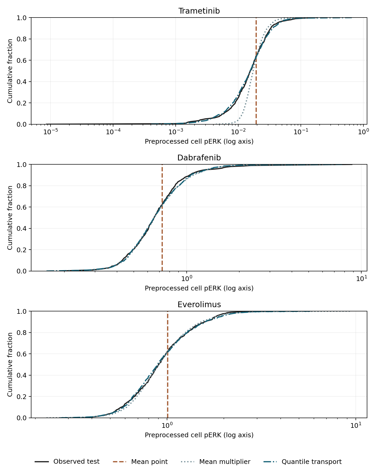
Figure 1. Marker CDFs. Black denotes treated evaluation cells, orange the mean point, gray mean scaling and blue quantile mapping. The vertical axis is the fraction at or below a value; preprocessed pERK is shown on logarithmic horizontal axes. Ranges differ by drug, so comparisons are within panels. Lines use 201 quantiles. The orange vertical line represents collapsing every cell to one value.
Wasserstein-1 distance measures distributional differences. In one dimension it integrates distances between quantiles:
\[ W_1(\mu,\nu)=\int_0^1|F_\mu^{-1}(u)-F_\nu^{-1}(u)|\,du. \]
Both mean error and \(W_1\) were divided by control-training standard deviation. Mean error is predicted minus observed mean; smaller distance indicates closer distributions. Distances use every evaluation value, rather than the 201 plotted quantiles.
Table 3. Mean errors and distributional distances in control-SD units
| Drug | Prediction | Mean error / control SD | W1 / control SD |
|---|---|---|---|
| Trametinib | Mean point | 0.0000 | 0.0260 |
| Trametinib | Mean multiplier | 0.0003 | 0.0109 |
| Trametinib | Quantile map | −0.0002 | 0.0036 |
| Dabrafenib | Mean point | −0.0694 | 0.6394 |
| Dabrafenib | Mean multiplier | −0.0605 | 0.1359 |
| Dabrafenib | Quantile map | −0.0644 | 0.1193 |
| Everolimus | Mean point | 0.0172 | 0.7979 |
| Everolimus | Mean multiplier | 0.0295 | 0.0762 |
| Everolimus | Quantile map | 0.0263 | 0.0687 |
For everolimus, the mean-point error was only 0.0172 but distance was 0.7979. Mean scaling had a slightly larger mean error yet reduced distance to 0.0762. Preserving spread matters in addition to predicting the mean.
Quantile mapping further reflects shape. This does not revalidate CMonge against other models: it is a custom single-marker diagnostic using an already measured treated distribution. Feature correlations and high-dimensional cell states were not reconstructed.
The reference distance between treated training cells themselves and treated evaluation cells was 0.0614 for everolimus in the main split. Quantile mapping's 0.0687 therefore also reflects differences between training and evaluation samples. This reference is neither an unseen-cell predictor nor a strict performance bound.
Upper-tail fractions and split sensitivity
Upper-pERK fractions were also examined. Drug-specific cutoffs were fixed at the treated training 90th percentile, without adjustment after examining evaluation cells.
Table 4. Fractions above the fixed training cutoff
| Drug | Observed upper-tail fraction | Mean multiplier | Quantile map |
|---|---|---|---|
| Trametinib | 7.77% | 4.87% | 10.19% |
| Dabrafenib | 9.53% | 11.51% | 10.19% |
| Everolimus | 10.02% | 8.59% | 10.19% |
All quantile-map fractions are near 10% because the map transfers training ranks. It does not discover an unknown high-marker population. For trametinib, 10.19% differs from the measured 7.77%; close overall distributions need not match a particular tail exactly.
There is no evidence identifying this upper tail as resistant cells. An eight-hour marker value does not establish subsequent survival, proliferation or response to repeat treatment. A resistance phenotype would require separate measurements linked to the marker classification.
Two additional splits retained smaller quantile-map distances than mean scaling for all three drugs, while magnitudes changed. Everolimus training–evaluation reference distances ranged approximately 0.044–0.143 across three splits. This is split sensitivity, not a confidence interval from independent biological replicates.
Discussion
Distributional evaluation does not by itself establish individual-cell transitions. Consider a separate four-point example: control and treated populations each place equal mass at −2, −1, 1 and 2. Pairing identical values or reversing their order leaves the same two observed distributions.
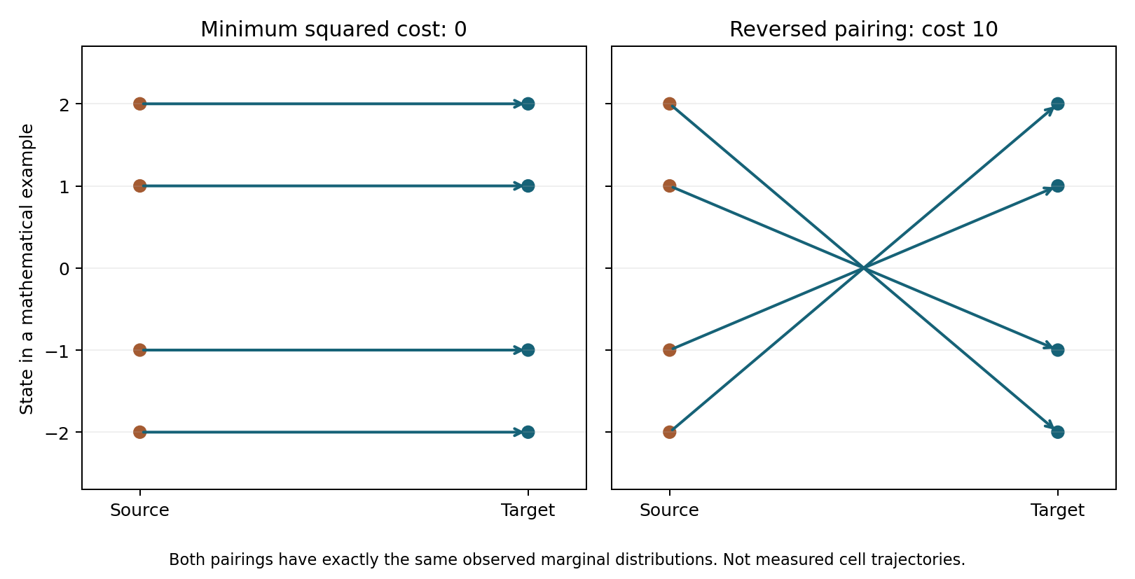
Figure 2. Mathematical pairing example, separate from measured data. Left: identical-value matching. Right: reversed matching. Mean squared transport costs are 0 and 10, and paired-state correlations are 1 and −1. Both have identical control and treated marginal distributions.
Squared-cost optimal transport selects the left pairing under a clear mathematical assumption. The two distributions do not establish that biology actually followed this minimum-cost pairing. Distributional fit and identification of individual histories are different properties.
The analysis normalizes measured cells to total probability one. Drug-induced cell loss or composition changes also affect the normalized distribution. Mapping alone cannot separate death, proliferation and state changes.
Conclusion
Marker means, distributional distances and upper-tail fractions captured different response features in these data. All are marginal-distribution metrics, however, and do not reconstruct same-cell histories or absolute counts. Known-condition cell splits also do not establish prediction for unmeasured drugs or independent experiments.
Data and code availability
The custom code, aggregate results, figures and reproduction instructions exclude original 4i files. fetch_data.py retrieves a fixed URL and verifies its hash. Python, NumPy, SciPy, h5py and matplotlib are required; analysis.py recalculates all three splits.
The exploratory scope was fixed after examining representative data values. Three drugs and one marker cannot establish generalization to new drugs, patients or experimental systems. Sources are the CellOT and CMonge papers, ETH record and benchmark distribution (1, 2, 3, 4). The package excludes third-party figures, papers, code, weights and individual cell identifiers.
References
- Bunne C, Stark SG, Gut G, del Castillo JS, Levesque M, Lehmann KV, et al. Learning single-cell perturbation responses using neural optimal transport. Nature Methods. 2023;20(11):1759–1768. doi:10.1038/s41592-023-01969-x.
- Driessen A, Rajwade DA, Harsanyi B, Rapsomaniki M, Born J. Conditional Monge Gap enables generalizable single-cell perturbation modelling. Nature Machine Intelligence. 2026;8(6):984–996. doi:10.1038/s42256-026-01242-8.
- Bunne C, Stark S, Gut G, Lehmann KV, Pelkmans L, Krause RA, et al. Datasets of Learning Single-Cell Perturbation Responses using Neural Optimal Transport [Dataset]. ETH Zurich; 2023 Apr 27. Data record.
- EntropicOTBenchmark contributors. EntropicOTBenchmark: single-cell drug 4i data [Research benchmark distribution]. Commit db2a4d0888e593659786fa27785c2fe1c82678fc [cited 2026 Oct 12]. Fixed files.