How complex does a population PK model need to be for exposure comparison? Measured nimotuzumab PK
Three population PK structures estimated from individual PK data, with internal validation, convergence and exposure differences across dosing conditions used to examine the limits of model selection.
Key findings
- Linear one-compartment, linear two-compartment and nonlinear-elimination PopPK models were fitted to public data (12 subjects, 321 concentrations). AIC fell with complexity (790.42, 751.25, 747.47), but leave-one-subject-out RMSE improved by only about 4.2% and 3.3%, short of the prespecified 10%.
- The 400 to 200 mg AUC ratio was 2 in the linear models and about 2.35 in the nonlinear model, a difference above 10%: the models ranked dosing conditions alike, but absolute exposure and dose ratios depended on the model.
- Only 4.5–22% of bootstrap runs passed the convergence screen, so no 95% CIs were reported. Adopting the nonlinear model and declaring the linear model sufficient are both deferred; original infusion and sampling records and independent validation data are needed next.
On this page
- Question and use
- Auditing the data first
- Estimating three candidates in the same framework
- Separating goodness of fit from prediction for new subjects
- VPC that preserves the dosing history
- Not forcing confidence intervals out of the bootstrap
- The same ranking of dosing conditions does not mean the same numbers
- What happens when the input-history and body-weight assumptions change
- What numerical checks confirmed
- What this analysis can decide
- Reproduction materials and sources
From published individual concentration data, I estimated three PopPK models: linear one-compartment, linear two-compartment, and two-compartment with nonlinear elimination. The analysis asks which structure is needed to compare exposure across dosing conditions, and how far the results can be trusted.
Here, the more complex models improved the fit to the training data. However, the improvement in internal validation with subjects left out was small, and convergence problems remained in resampling-based estimation. Although the models ranked the dosing conditions in the same order, absolute exposure and dose ratios did not agree. The evidence was therefore insufficient either to adopt the nonlinear model or to conclude that the linear model is enough. This article shows the calculations behind that conclusion and the information needed next.
Question and use
In the original nimotuzumab study, a semi-mechanistic nonlinear PK model was examined for data from patients with advanced breast cancer.[1] This analysis is not a full reproduction of the original model. It is a secondary analysis that uses the data distributed in a public package to compare model complexity against the intended use.
- QOI: For repeated doses of 50–400 mg, how much do exposure at the first and tenth doses, and the comparison between dosing conditions, change when the model structure changes?
- COU: Research and learning comparisons of exposure with public data, and examination of whether structure is needed and what additional measurements to make.
- Out of scope: Selection of therapeutic doses, prediction of individual safety or efficacy, EGFR occupancy, dose decisions for clinical trials.
"Ranking in the same order" and "agreeing numerically to the precision needed for the use" are different judgments. The analysis plan required, as conditions supporting added complexity, an improvement of at least 10% in subject-level prediction RMSE together with calibration and identifiability. To conclude that a simpler structure is enough, it required that the main exposures and ratios differ by no more than 10% from plausible alternative models, together with an assessment of uncertainty. This 10% is a prespecified criterion for this study, not a general regulatory standard.
Auditing the data first
nimoData from nlmixr2data 2.0.10 at a fixed commit was used.[2] The SHA-256 of the original RDA is 896d256aee8919061b76358c5e723a786571182f88e5069bf5aa79fc24b82352. The RDA was written out to CSV, and dosing and observation records were checked separately.
| Item | Distributed content and handling |
|---|---|
| Subjects | 12; 3 each at 50 / 100 / 200 / 400 mg |
| Events | 441 rows: 120 doses and 321 concentration observations |
| Repeated dosing | 10 doses for everyone; actual TIME used continuously |
| DV | Natural-log concentration; exp(DV) is in µg/mL (equivalent to mg/L) |
| Time, dose, rate | h, mg, mg/h |
| Infusion duration | 0.37–2.91 h from the recorded AMT/RATE; correspondence with the nominal 0.5 h of the original study is unresolved |
| TAD | Inconsistent with the time since the previous dose in 143/321 observations; not used in the ODE |
| BLQ | No dedicated flag; whether unrecorded BLQ values exist cannot be determined |
| Independent information | Not 321 rows but, first of all, 12 people; 3 independent subjects per dose |
The log scale is consistent with IPRED = log(conc) in the official model example.[3] DV = 0 in dosing rows is not mixed with concentration observations. The recorded dosing intervals were 93.0–312.6 h and were not rounded to the nominal 168 h for estimation.
The audit of the original paper (A01) recorded 443 concentration observations, but the distributed data contain 321, and there is no table mapping extraction or processing.[1,2] The analysis uses the 321 distributed observations; it cannot be described as reproducing the full data of the original study. Estimation used the recorded RATE, and replacing all infusions with 0.5 h was re-estimated as a separate sensitivity analysis.
Estimating three candidates in the same framework
Let concentration be C = A1 / V1 and the infusion input R_in(t). M1 is a linear one-compartment model, and M2 is the following linear two-compartment model.
\[ \frac{dA_1}{dt}=R_{\mathrm{in}}(t)-CL\,C-Q\frac{A_1}{V_1}+Q\frac{A_2}{V_2},\qquad \frac{dA_2}{dt}=Q\frac{A_1}{V_1}-Q\frac{A_2}{V_2}. \]
M3 adds the following Michaelis–Menten term to central elimination in M2.
\[ \frac{dA_1}{dt}=R_{\mathrm{in}}(t)-CL\,C-Q\frac{A_1}{V_1}+Q\frac{A_2}{V_2} -\frac{V_{\max}C}{K_m+C}. \]
M1 omits Q and the peripheral compartment. In all three candidates, log-normal between-subject variability (IIV) was placed on CL and V1, with the covariance fixed at 0.
\[ CL_i=CL_{\mathrm{pop}}\exp(\eta_{CL,i}),\quad V_{1,i}=V_{1,\mathrm{pop}}\exp(\eta_{V,i}),\quad \eta_i\sim N(0,\Omega). \]
The residual was additive error on log concentration.
\[ y_{ij}=\log\{C_i(t_{ij})+10^{-12}\}+\epsilon_{ij},\qquad \epsilon_{ij}\sim N(0,\sigma^2). \]
Km in M3 is not the EGFR binding affinity or receptor occupancy, and it differs from the TMDD model in the official example. The nonlinear term here is a candidate structure for describing the PK curve and is not interpreted as identifying a biological mechanism.
Estimation used R 4.5.1, nlmixr2est 7.1.0 and rxode2 5.1.8. In A02, SAEM was run from three starting points each, and M2/M3 were refined with FOCEi from three starting points each. Because differences due to the likelihood integration settings were detected, AIC was compared on the same data scale with independent adaptive Gauss–Hermite quadrature (25 points); the difference from 15 points was also saved. Re-estimation in A03 used FOCEi with limits of 1000 outer / 300 inner iterations and ODE atol 1e-9 and rtol 1e-6.[4]
The estimates of the selected candidate solutions are shown below. CL/Q are in L/h, V1/V2 in L, Vmax in mg/h and Km in µg/mL. Values are on the natural scale after exponentiation. sigma is the SD of log concentration, and omega is the variance of the log parameter.
| Model | CL | V1 | Q | V2 | Vmax | Km | sigma | omega_CL | omega_V1 |
|---|---|---|---|---|---|---|---|---|---|
| M1 | 0.008629 | 1.775 | — | — | — | — | 0.7459 | 0.2394 | 0.2786 |
| M2 | 0.003797 | 1.47 | 0.004676 | 60.65 | — | — | 0.7035 | 0.8028 | 0.2611 |
| M3 | 0.001595 | 1.473 | 0.001861 | 8.279 | 2.372 | 396.7 | 0.6932 | 2.133 | 0.2803 |
With a common likelihood, AIC was 790.42 for M1, 751.25 for M2 and 747.47 for M3; M3 is about 3.78 lower than M2. However, in A02 the largest absolute parameter correlation for M3 was about 0.990, and covariance and optimizer warnings remain. The model is not adopted on the AIC ranking alone.
Separating goodness of fit from prediction for new subjects
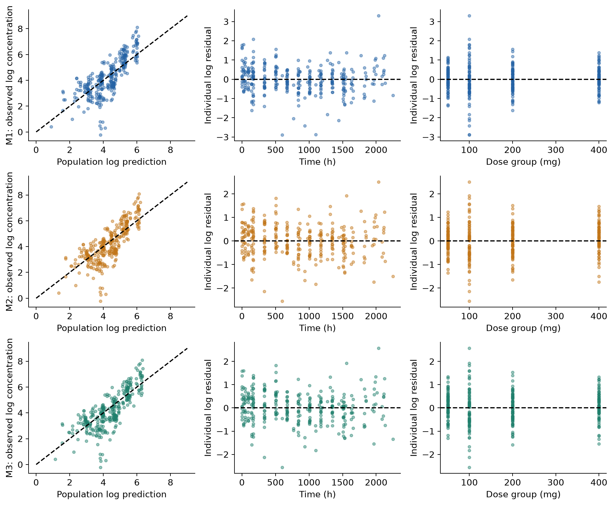
Figure 1. PRED against DV for the training data, and IRES against time and dose, on a log scale. IRES are residuals after individual effects are estimated and show fit to the training data. This is not independent predictive validation.
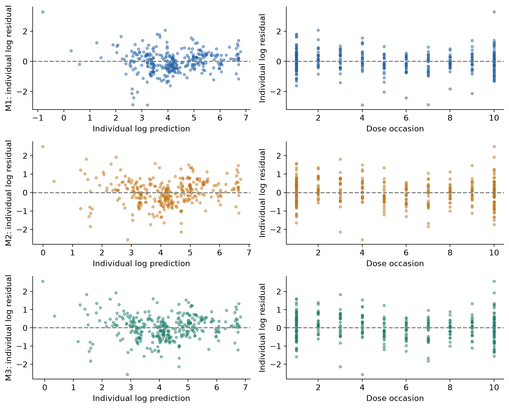
Figure 2. IRES against IPRED and dosing occasion. A simple mean residual can miss biases that depend on time or repeated dosing, so this is checked together with Figure 1.
The degree to which individual effects shrink toward 0 was also checked. Eta shrinkage defined on the SD scale is shown below (%). Values defined on the variance scale were saved to a CSV; the two definitions are not mixed. Low shrinkage does not guarantee identifiability or predictive validity of a model.[5]
| model | parameter | SD_shrinkage |
|---|---|---|
| M1 | eta.cl | 0.3 |
| M1 | eta.v | 4.792 |
| M2 | eta.cl | 5.921 |
| M2 | eta.v | 7.557 |
| M3 | eta.cl | 13.75 |
| M3 | eta.v | 6.2 |
Subjects were left out one at a time, and the fixed effects, IIV and residual were re-estimated from the remaining 11 (LOSO, 12 folds). Individual effects were not estimated from the left-out subject's DV; the marginal prediction integrating over IIV was evaluated, using a Monte Carlo approximation with 2048 draws per fold. The table gives log-concentration RMSE, coverage and pointwise log predictive density calculated for each subject and averaged over the 12 subjects with equal weight. The predictive density is not the joint density of all repeated observations.
| model | RMSE | RMSE improvement vs M1 (%) | coverage | mean_lpd |
|---|---|---|---|---|
| M1 | 0.9458 | 0 | 0.9186 | -1.386 |
| M2 | 0.9061 | 4.195 | 0.9218 | -1.347 |
| M3 | 0.9147 | 3.288 | 0.9189 | -1.332 |
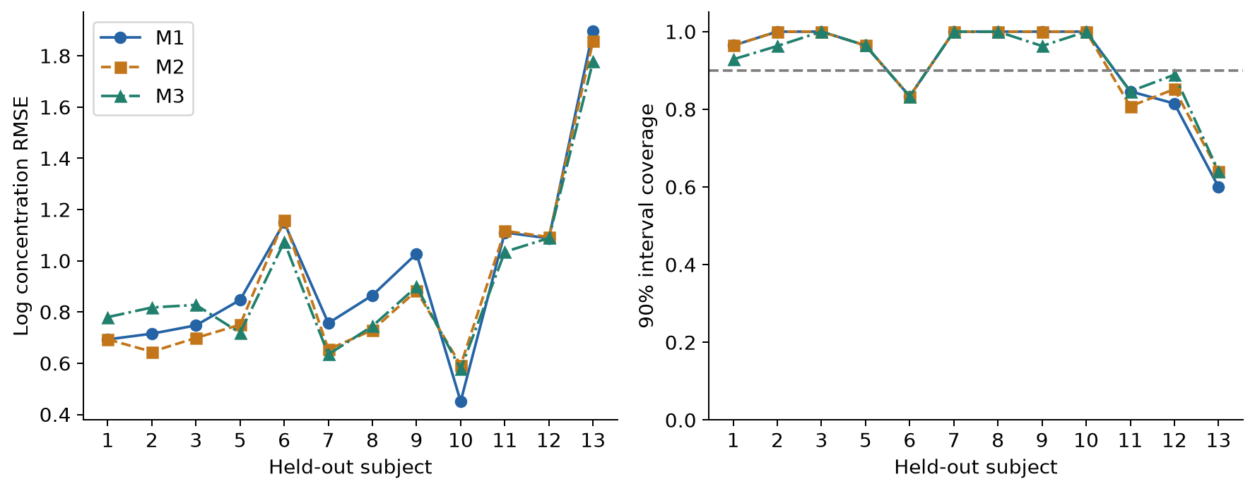
Figure 3. RMSE and coverage of the 90% prediction interval by model for the same subjects. Connected points show the pairing. Subjects with many observations are not given extra weight.
The mean improvement for M2/M3 does not reach 10%. With an 8192-point Sobol integration using a different seed, the improvements were 4.10% and 3.16%, and the judgment did not change. However, this result is not taken to conclude that added complexity is unnecessary. Convergence warnings remain in LOSO, and as the table below shows, not all folds passed the convergence screen. The metrics in the table are an exploratory internal diagnostic using all finite solutions. Because starting values chosen on the full data were used, this is neither nested validation including model selection nor external validation.
| Model | Folds | Finite | Pass convergence screen |
|---|---|---|---|
| nlminb-M1 | 12 | 12 | 5 |
| M2 | 12 | 12 | 0 |
| M3 | 12 | 12 | 1 |
VPC that preserves the dosing history
Actual dosing times, rates and sampling times were kept, and 1000 datasets were generated for each model. The same eta was used for repeated observations of the same subject, with residual error added to each observation. The first and tenth doses were separated by dose level and summarized by time since the previous dose. The time bins were 0–2, 2–30, 30–72, 72–168, 168–360 and 360–720 h, set to cover the recorded schedule; bins with fewer than 3 observations are not shown.
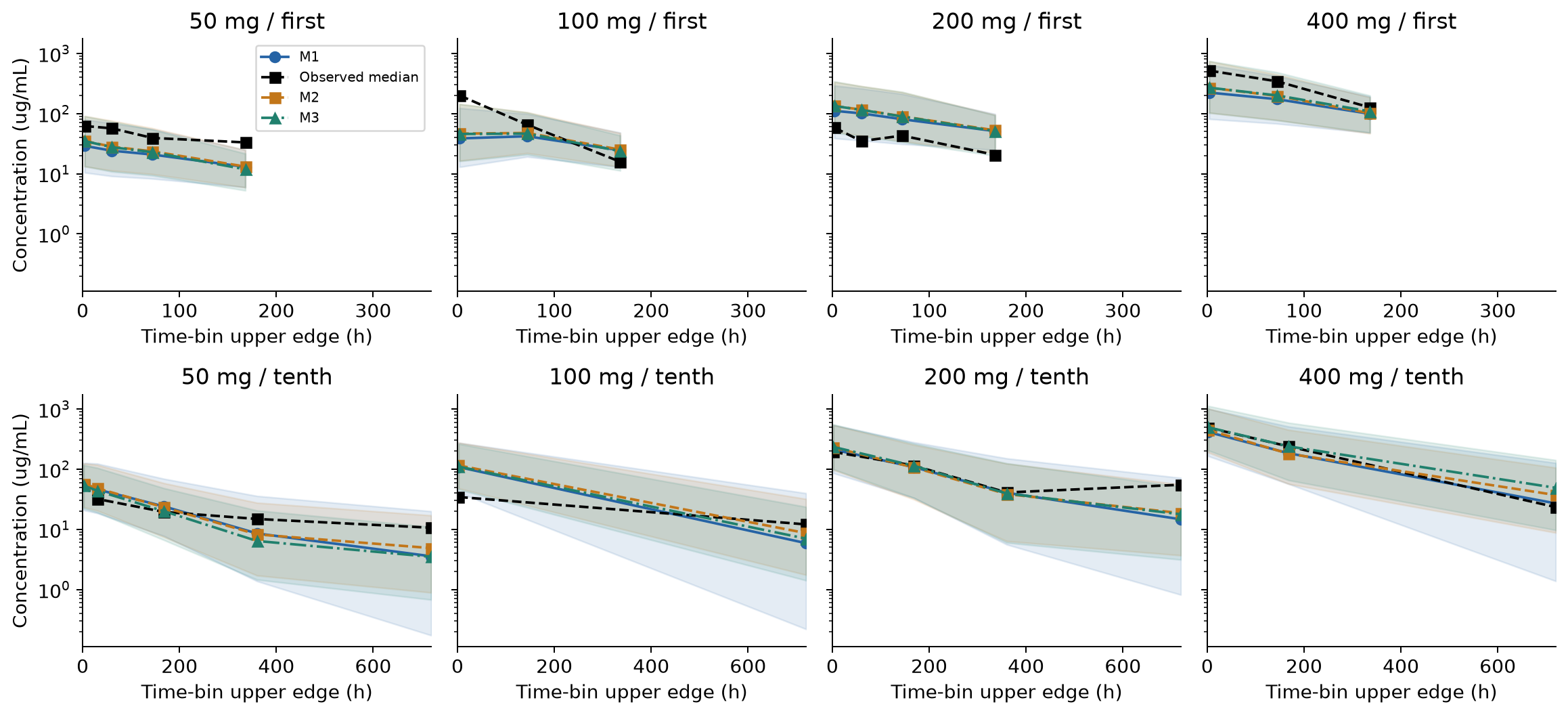
Figure 4. Black is the observed median, colored lines are the median of the replicate simulations, and bands are the 90% simulation interval of the median in each bin. The vertical axis is log concentration and the horizontal axis is the upper edge of the bin, not the sampling times themselves. The 10th/50th/90th percentiles were saved in the full VPC output, but the figure shows only medians. The bands are neither the 90% interval of the between-subject distribution nor a confidence interval for parameters.
With three subjects per dose, several observations in a bin do not add independent subjects. Medians are shifted for some doses and periods, and inclusion within a wide band alone does not guarantee fit. This is an uncorrected VPC by dose, not a prediction-corrected VPC.
Not forcing confidence intervals out of the bootstrap
Keeping the dose strata, subjects were resampled with replacement and each model was re-estimated 200 times. Observation rows were not resampled individually. Because this is the empirical distribution of strata with only three people, the lack of information in a small population remains. For M1, the optimizer was changed from bobyqa to nlminb and another 200 runs were made. The additional runs did not replace the original results; both were kept.
| group | attempted | finite | qualified | qualified_rate | CI_defensible |
|---|---|---|---|---|---|
| M1 | 200 | 200 | 9 | 0.045 | False |
| M2 | 200 | 200 | 9 | 0.045 | False |
| M3 | 200 | 200 | 11 | 0.055 | False |
| nlminb-M1 | 200 | 200 | 44 | 0.22 | False |
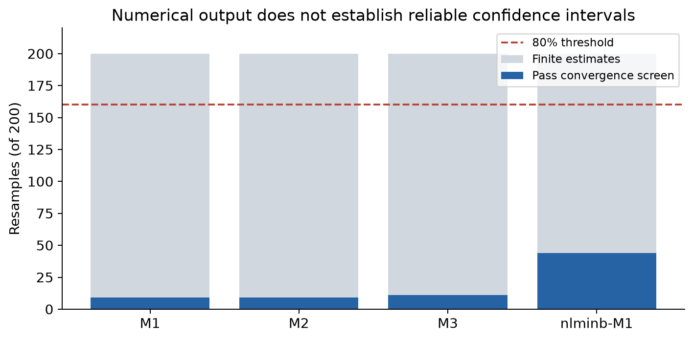
Figure 5. Gray is the number of runs with finite estimates, and blue is the number that passed the specified convergence screen. All records related to not at minimum, maximum iterations, failure and convergence were checked. Because runs that pass may still carry notes such as gradient warnings, the number passing is not interpreted as the number of fully warning-free successes.
No candidate reaches the prespecified 80% criterion, so 95% confidence intervals from this bootstrap are not reported. Building intervals from only the few successful runs would give a distribution that excludes the data configurations that fail. The finite outputs, convergence records and estimates themselves were saved for audit.
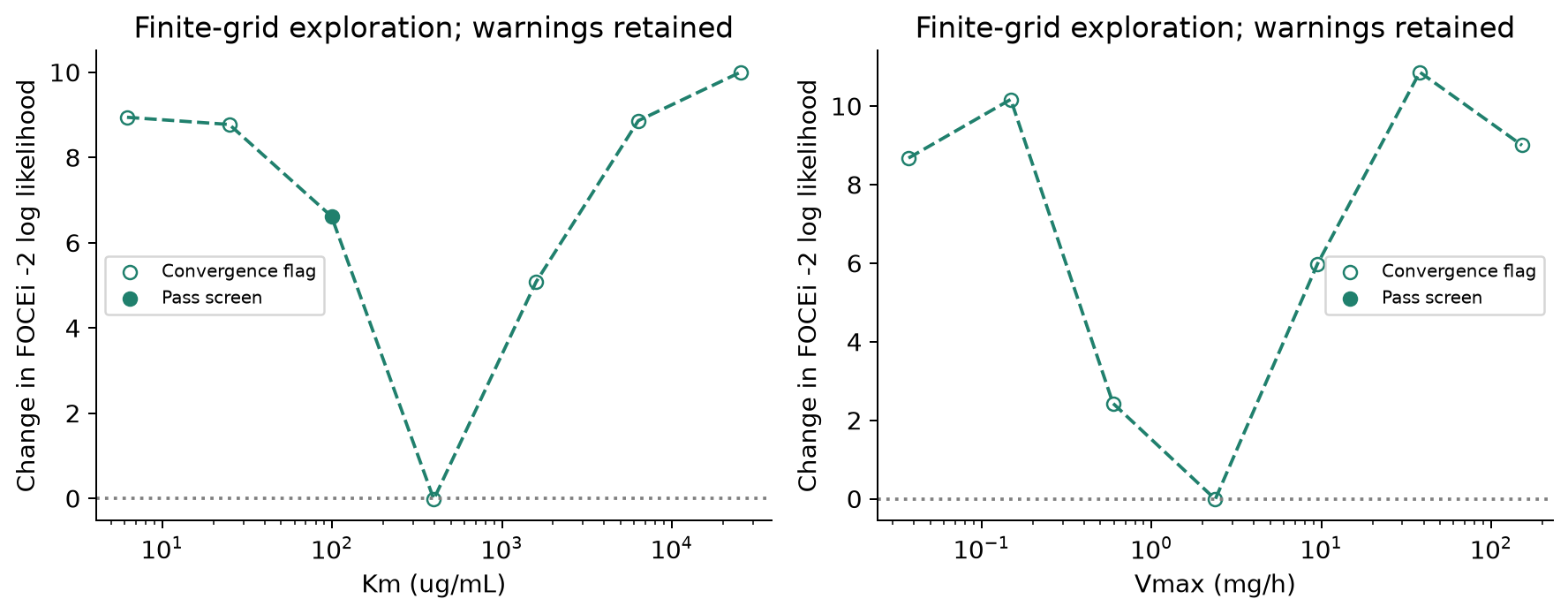
Figure 6. Km or Vmax was fixed at 1/64 to 64 times the candidate solution (7 points), and the remaining parameters were re-estimated. The vertical axis is the difference from the A03 reference FOCEi objective function. This is a finite grid search, not the independent-quadrature curve used for AIC and not a formal profile confidence interval. Points with convergence warnings are shown as open symbols rather than hidden. The curve is not taken as a smooth true profile, and the boundedness of an interval is not asserted.
The same ranking of dosing conditions does not mean the same numbers
Estimation used the actual dosing history. For the comparison simulations, conditions were standardized: 50 / 100 / 200 / 400 mg, a 168 h interval, a 0.5 h infusion and 10 doses. Fixed effects were set to the candidate solutions, and 10,000 people following each model's Omega were generated from the same standard normal random numbers. Within each model, this is a paired comparison giving every condition to the same virtual individuals. Using the same random numbers across models does not guarantee the same biological individual differences in the same real patient.
From the concentrations, AUC, Cmax, Ctrough and Cavg were calculated for the first dose (0–168 h) and the tenth dose (1512–1680 h). The tenth dose is not called steady state. Cmax is the maximum on an evaluation grid that includes the end of infusion, and AUC is a numerical integral. Residual error was not added to exposure simulations that show IIV.
The table gives the 10th/50th/90th percentiles of tenth-dose AUC (µg·h/mL) and the median of each virtual individual's ratio to the 200 mg condition. "The ratio of medians" and "the median of individual ratios" are distinguished.
| model | amount_mg | p10 | median | p90 | Paired median ratio vs 200 mg |
|---|---|---|---|---|---|
| M1 | 50 | 3102 | 5781 | 1.046e+04 | 0.25 |
| M1 | 100 | 6205 | 1.156e+04 | 2.092e+04 | 0.5 |
| M1 | 200 | 1.241e+04 | 2.312e+04 | 4.184e+04 | 1 |
| M1 | 400 | 2.482e+04 | 4.625e+04 | 8.369e+04 | 2 |
| M2 | 50 | 3107 | 6213 | 9010 | 0.25 |
| M2 | 100 | 6213 | 1.243e+04 | 1.802e+04 | 0.5 |
| M2 | 200 | 1.243e+04 | 2.485e+04 | 3.604e+04 | 1 |
| M2 | 400 | 2.485e+04 | 4.97e+04 | 7.208e+04 | 2 |
| M3 | 50 | 2891 | 5905 | 7086 | 0.2141 |
| M3 | 100 | 5879 | 1.248e+04 | 1.534e+04 | 0.4524 |
| M3 | 200 | 1.212e+04 | 2.758e+04 | 3.563e+04 | 1 |
| M3 | 400 | 2.541e+04 | 6.497e+04 | 9.158e+04 | 2.351 |
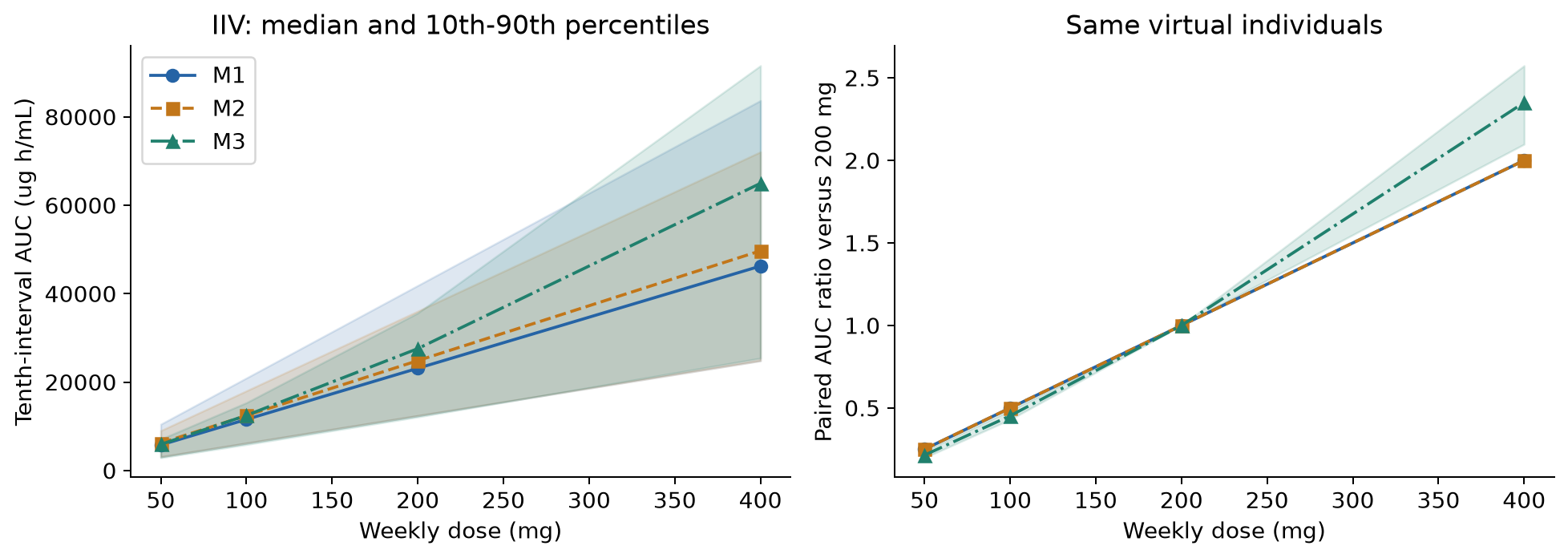
Figure 7. Left: median and 10th–90th percentiles of AUC from IIV. Right: AUC ratios within the same virtual individuals. The bands are not confidence intervals for parameter estimates.
In M1/M2, linearity makes the 400 mg to 200 mg AUC ratio exactly 2. The paired median for M3 was about 2.35. This difference in ratio exceeds the prespecified 10% criterion. On the other hand, M3 retains problems with identification of the nonlinear term and stability of re-estimation. It therefore cannot be concluded either that "2.35 is the correct dose ratio" or that "the linear 2 is enough". What can be supported here is that the model dependence was confirmed.
Ten doses of 200 mg at intervals of 144 / 168 / 192 h were also compared. The total dose is the same but the total duration differs, so Cavg over the tenth interval is compared in addition to AUC. Higher concentrations with shorter intervals are not to be read as a safety or efficacy advantage.
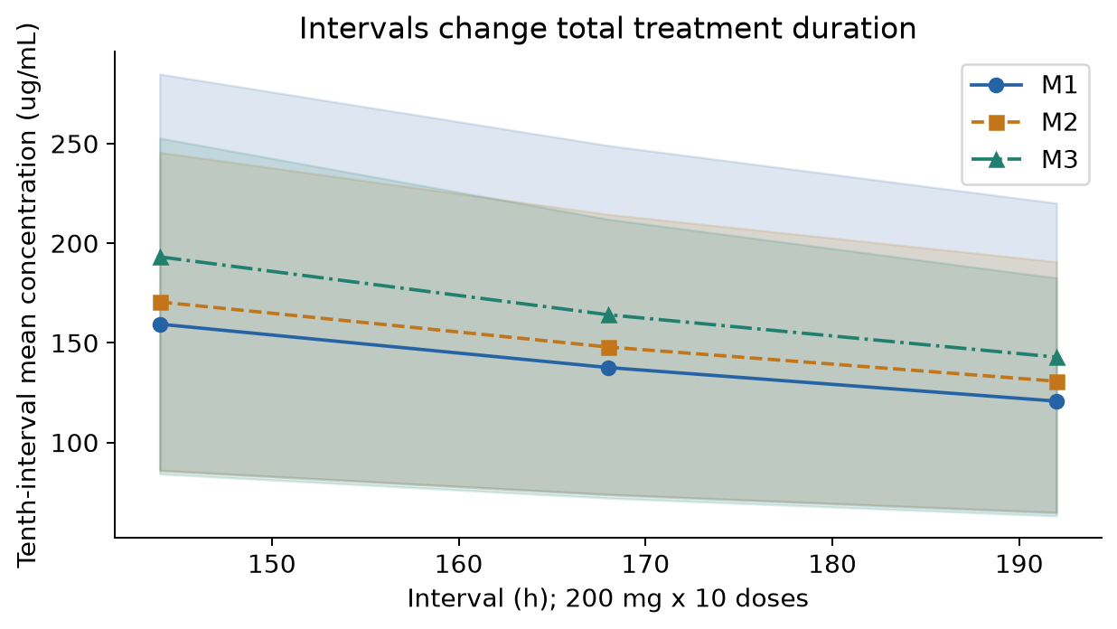
Figure 8. Median and 10th–90th percentiles from the IIV of each candidate solution. The length of the tenth interval itself differs by condition. Uncertainty in the fixed-effect estimates is not included in the bands.
With the same parameters, changing a 0.5 h infusion to 1 h changed the paired median of first-dose Cmax by about −0.1% to −0.2% in all three models. This is a comparison in which "only the infusion was changed with the same pharmacokinetics", which differs from the input-history sensitivity below.
What happens when the input-history and body-weight assumptions change
Exposure from the solutions re-estimated with subjects left out was also examined. The table gives the range across the 12 leave-one-out solutions of the typical-individual tenth-dose AUC at 200 mg and the 400/200 mg ratio. These are neither between-subject distributions nor confidence intervals.
| model | endpoint | minimum | maximum | screen_pass_folds |
|---|---|---|---|---|
| M1 | typical_AUC200 | 2.126e+04 | 2.513e+04 | 5 |
| M1 | typical_ratio400_200 | 2 | 2 | 5 |
| M2 | typical_AUC200 | 2.342e+04 | 2.723e+04 | 0 |
| M2 | typical_ratio400_200 | 2 | 2 | 0 |
| M3 | typical_AUC200 | 2.558e+04 | 3.113e+04 | 1 |
| M3 | typical_ratio400_200 | 2.187 | 2.466 | 1 |
The M3 dose ratio stayed at about 2.19–2.47 when subjects were left out one at a time, different from the linear value of 2. However, only 1 of the 12 M3 solutions passed the convergence screen. This is kept as a sensitivity check of whether a single subject changes the result, not as a robust population prediction. The leave-one-out Km/Vmax solutions were saved in a separate CSV.
A re-estimation replacing all recorded infusions with 0.5 h, and a re-estimation with fixed allometry using baseline body weight (CL exponent 0.75, V1 exponent 1, reference 70 kg), were saved separately from the original candidates. The exponents were not estimated. The table gives the typical-individual tenth-dose AUC for 200 mg weekly, 10 doses, 0.5 h infusion, for each re-estimated solution. Allometry is compared at 70 kg.
| group | allometry-fixed | baseline | infusion-0.5h | infusion-0.5h / baseline | allometry-fixed / baseline |
|---|---|---|---|---|---|
| M1 | 2.164e+04 | 2.299e+04 | 2.293e+04 | 0.9973 | 0.9412 |
| M2 | 2.406e+04 | 2.483e+04 | 2.499e+04 | 1.007 | 0.9693 |
| M3 | 2.759e+04 | 2.751e+04 | 2.797e+04 | 1.017 | 1.003 |
| nlminb-M1 | 2.159e+04 | 2.317e+04 | 2.28e+04 | 0.9839 | 0.9319 |
Because convergence warnings also remain for each sensitivity re-estimation, the differences are not treated as proof of a robust covariate effect or of the correct infusion duration. In addition, exposure including body weight and IIV was calculated for 10,000 people with recorded baseline weights resampled with replacement (allometry-exposure.csv). This is a sensitivity analysis conditional on the weight distribution of the 12 observed people, not the distribution of a general patient population. It does not claim to have synthesized the joint distribution of unknown patient characteristics.
What numerical checks confirmed
An independent Python implementation (analytical transitions for the linear models, DOP853 for M3) was compared with the R predictions for nine estimated solutions covering the reference, infusion sensitivity and allometry. The maximum difference in log prediction was 3.3e-06. Changing the integration grid from 337 to 673 points changed AUC by at most 3.6e-07 in relative terms (a cohort of 32 people with the same random numbers). It was also confirmed that the paired dose ratios for M1/M2 match the theoretical linear values, that LOSO covered 36 subject folds and 963 observation evaluations, and that the exposure table has 168 rows.
These are checks of the implementation and numerical integration. They do not resolve the provenance of the data, the convergence of estimation, or the biological validity of the model.
What this analysis can decide
| Judgment | What is supported here | What is not supported |
|---|---|---|
| PopPK with measured data | Estimated and compared three candidates including between-subject variability | Full reproduction of the whole original study |
| Adding structure | Training fit improves, but prediction improvement is small and instability remains | Confirming adoption of the nonlinear model |
| Sufficiency of the linear model | Usable as a simple reference for comparison | Guaranteeing that dose ratios and absolute exposure are accurate enough |
| Comparing dosing conditions | Exposure and ratio differences within fixed candidate models can be quantified | Optimizing therapeutic doses, predicting clinical risk |
| Uncertainty | IIV, structural differences and re-estimation failures can be distinguished | Reliable 95% CIs from the bootstrap |
What is needed next is not simply adding another complex equation. First, the original records of infusion start and end and sampling times, and the history of selecting and processing the distributed data, should be checked. Then measurements that can distinguish the early distribution phase from the low-concentration terminal phase, more independent subjects per dose, and validation data not used for selection are needed.
If additional measurements are designed for existing data, the next question is to weigh the differences between candidate-model predictions in the low and high concentration ranges against measurement error and sampling burden. This analysis alone has not determined optimal sampling times or the required number of subjects, so no specific design values are proposed.
Reproduction materials and sources
The analysis record is saved in the executed a03-diagnostics.ipynb. For distribution, a review notebook that runs without patient-level data, instructions for rerunning, model definitions and R re-estimation scripts, independent Python prediction, diagnostics and simulation, summary CSVs and figures were prepared. The review notebook reruns the comparisons and checks from saved results; the long R estimation itself is a separate command. The distribution materials contain no patient-level data or RDS files and record the source of the fixed version and the hash of the original. The license for the code is treated separately from the usage rights for the original data and the copyright of the original paper.
- Rodríguez-Vera L, et al. Semimechanistic model to characterize nonlinear pharmacokinetics of nimotuzumab in patients with advanced breast cancer. J Clin Pharmacol. 2015;55:888–898. DOI:10.1002/jcph.496. Author-shared full text audited in A01.
- nlmixr2data: the fixed commit used in the analysis. Package 2.0.10; the hash of the original is given in the text.
- Official nlmixr2 nimotuzumab example. Reference for the data scale and the original study model. M3 here is not described as a reproduction of that TMDD model.
- Official nlmixr2est foceiControl reference. Optimizer and estimation control.
- Savic RM, Karlsson MO. Importance of shrinkage in empirical Bayes estimates for diagnostics: problems and solutions. AAPS J. 2009;11:558–569. DOI:10.1208/s12248-009-9133-0, open full text.
The tables and figures in this article were created from this analysis of the distributed data. No figures from the cited papers are reproduced.
Complete analysis materials (code, summary results, executed notebooks)
Cite this article
Kumakura, D. (2026). How complex does a population PK model need to be for exposure comparison? Measured nimotuzumab PK. daikikumakura.github.io. https://daikikumakura.github.io/writing/nimotuzumab-poppk-en.html