Does separating PSA decline and regrowth improve early prediction?
A public clinical PSA dataset used to compare landmark prediction, uncertainty calibration and decline/regrowth identifiability against simple benchmarks.
Key findings
- In 400 patients from a public PSA dataset, a decline–regrowth hierarchical model predicted the next 12 weeks of PSA better than linear or single-decay models at every landmark (MAE 0.429 vs 0.543–0.565 at 6 weeks).
- Its advantage over simply carrying the last PSA value forward was uncertain at 6 and 12 weeks, and at 24 weeks the last value was more accurate (MAE 0.249 vs 0.327).
- The regrowth rate was weakly identified, with its population mean at the lower bound at every landmark, so no minimum observation period for a regrowth-based decision can be set from these data.
On this page
- Summary
- 日本語要旨
- Question and context of use
- Public data and the audit that changed the analysis
- Models: separate the shape from the estimation method
- Prediction design
- Results: a complex model needs a strong simple benchmark
- Calibration is not the same as a narrow interval
- Identification: the prior must not supply the conclusion
- Sensitivity: shrinkage and treatment boundaries matter
- What can be decided?
- Limits and reproducibility
- References
Summary
A curve can fit PSA measurements without identifying a distinct regrowth rate. It can also outperform an overly rigid decay model while adding little to the latest observed PSA. Those are different claims and require different checks.
Using 400 patients in a public PSA/survival example dataset, I compared early predictions from a constant last value, a linear hierarchy, a single-decay model, and a decline–regrowth hierarchy. Each prediction used only the patient's history available at 6, 12, 18 or 24 weeks. The target was the observed, uncensored, on-treatment PSA in the following 12 weeks.
The two-component model improved on the fitted linear and single-decay candidates. Its advantage over the last-value benchmark was uncertain at 6 and 12 weeks; at 24 weeks the last value was better in the paired test-cohort comparison. Regrowth remained weakly informed under the implemented approximate hierarchical estimator, with its population mean at the lower parameter bound at every landmark. This is a failure to qualify a regrowth-based early decision rule, rather than evidence that regrowth never occurs.
日本語要旨
登録不要で取得できる400人のPSA実測データから、低下・再上昇を分けた階層モデルを推定し、患者を学習・区間校正・検証に分けて早期予測を評価した。2成分モデルは単純な低下モデルより予測誤差が小さかったが、直近値を使う予測に対する優位性は初期時点では明確ではなく、24週では直近値の方が良好だった。再上昇速度の情報も弱かった。今回の近似推定法と評価対象において、「複雑なモデルを使えばよい」「何週あれば再上昇を判断できる」とは結論できない。予測精度、速度の識別性、治療継続者への選択を分けて判断する必要がある。
Question and context of use
Question: how much observation is needed before separating PSA decline and regrowth adds reliable predictive information beyond simple extrapolation?
Context of use: retrospective evaluation of measurement and modeling design. The analysis does not select an individual treatment, compare drug effects, estimate resistant-cell fractions, or qualify PSA as an overall-survival surrogate. A negative result is useful if it prevents a convenient fitted parameter from becoming an unsupported decision rule.
The relevant comparison is an honest prediction benchmark at the same landmark. Fitting all available follow-up and then claiming an early prediction would answer a different question.
Public data and the audit that changed the analysis
The official downloadable example contains 400 patients, 6,627 PSA rows and 286 deaths. It is the original publication's training subset from the VENICE comparator treated with docetaxel/prednisone. The separate original validation subset is not included in this download. I split the 400 again for internal evaluation; this is not external validation. Desmée et al., 2017
Three details matter before fitting:
- The supplied observation is transformed. The CSV's PSA values are on the natural-log
log(PSA+1)scale, consistent with the original observation equation. All 165 below-quantification rows equallog(1.1), matching the documented 0.1 ng/mL threshold. Treating that column as raw ng/mL would fit the wrong model. - Repeated dates are not identical duplicates. Two same-day PSA groups contain slightly different values. I average each group on the supplied transformed scale, leaving 6,625 distinct patient/date PSA records. I do not silently keep one arbitrary value.
- Treatment time and survival are separate records. The CSV includes treatment-end time and two survival rows per patient: a time-zero record and a final event/censoring record. PSA after treatment end is excluded from the main target. It remains available for a separate sensitivity analysis.
The original protocol scheduled PSA approximately every 21 days during treatment and every 84 days afterwards. Actual visit times are used rather than forcing measurements onto those schedules. Pre-treatment records are retained for the audit but excluded from this on-treatment shape model. Original methods
The raw CSV is publicly offered without account registration. It is not bundled with the companion: public availability does not establish unrestricted redistribution rights. The acquisition script downloads the official file and checks its recorded SHA256. All figures here are original aggregate figures.
Models: separate the shape from the estimation method
Let the latent on-treatment PSA be
\[ S_i(t)=B_i\left[A_i e^{-d_i t}+(1-A_i)e^{g_i t}\right], \qquad 0<A_i<1,\ d_i,g_i>0, \]
and the observation model be
\[ y_{ij}=\log\{1+S_i(t_{ij})\}+\epsilon_{ij}. \]
Dividing the latent response by \(B_i\) gives exactly one at time zero. This avoids doubling the baseline by summing two unweighted exponentials. Estimating a latent baseline also avoids treating every noisy ratio to the first measurement as independent.
The transformed parameters \(z_i=(\log B_i,\log d_i,\log g_i,\operatorname{logit}A_i)\) have a diagonal Gaussian hierarchy. The comparator candidates are the latest measured value, a hierarchical linear predictor on the supplied scale, and a single exponential decline. Here \(d\), \(g\) and \(A\) describe PSA shape; they are not directly measured tumor-cell growth, mutation or resistant fractions.
The estimator is deliberately explicit about its approximation. Population parameters maximize a first-order Gaussian marginal likelihood,
\[ f(z_i,t)\approx f(\mu,t)+J(\mu,t)(z_i-\mu), \qquad V_i=J_i\operatorname{diag}(\omega^2)J_i^\top+\sigma^2I. \]
The linear candidate has an exact Gaussian marginal likelihood; the nonlinear candidates use a Taylor approximation. Individual predictions use nonlinear empirical-Bayes MAP estimation. This is neither SAEM nor exact nonlinear marginal maximum likelihood, and it does not reproduce the original mechanistic ODE/survival model. Three population starts, optimizer diagnostics and numerical bounds are supplied with the results.
Population fitting uses uncensored measurements. Individual MAP calculations include a Gaussian CDF contribution for below-quantification observations. This hybrid is a limitation: an individual censoring term does not make the population estimator a fully censored NLME likelihood. Predictive checks and sensitivity analyses are needed before relying on it, and parameter qualification would require a more complete estimator.
Prediction design
The split is fixed at 240 training, 80 calibration and 80 test patients, using seed 20261004. For each landmark, eligibility requires continued treatment and follow-up plus at least two prior on-treatment PSA measurements spanning 14 days. Population fitting uses only eligible training patients and their history through that landmark. Test predictions use each test patient's prior history; their future measurements do not enter fitting.
The main target is an observed-target window: uncensored PSA measured while still on treatment during the next 84 days. It is not an exact visit-time target, and it does not represent patients with no subsequent measurement. Errors are calculated within patient and then averaged across patients, so frequent measurement does not make one patient dominate the MAE.
For prediction intervals, each calibration patient contributes one score: the largest absolute prediction error over that patient's observed target window. The finite-sample 90% split-conformal quantile gives a common radius on the supplied scale. Test coverage means all the patient's observed targets fall inside their intervals. It is separate from per-measurement coverage. This construction requires exchangeability of selected calibration/test patients and does not give a guarantee for missing measurements or after a shift in clinical setting. Angelopoulos and Bates
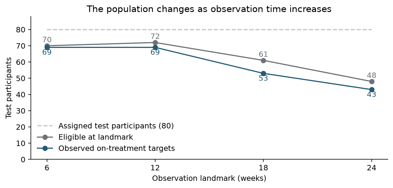
Figure 1. The denominator changes with landmark. Of the assigned 80 test patients, 69, 69, 53 and 43 contribute main prediction targets. Falling error over time therefore cannot be attributed solely to gaining more observations; later assessment also selects a different treatment-continuing population.
Results: a complex model needs a strong simple benchmark
All MAEs below are in log(PSA+1) units and are patient-weighted. They are not ng/mL errors, percentages or response probabilities.
| Landmark | Test patients / targets | Last value MAE | Linear MAE | Decay MAE | Two-component MAE |
|---|---|---|---|---|---|
| 6 weeks | 69 / 234 | 0.472 | 0.543 | 0.565 | 0.429 |
| 12 weeks | 69 / 213 | 0.395 | 0.536 | 0.511 | 0.365 |
| 18 weeks | 53 / 163 | 0.325 | 0.583 | 0.555 | 0.354 |
| 24 weeks | 43 / 118 | 0.249 | 0.515 | 0.477 | 0.327 |
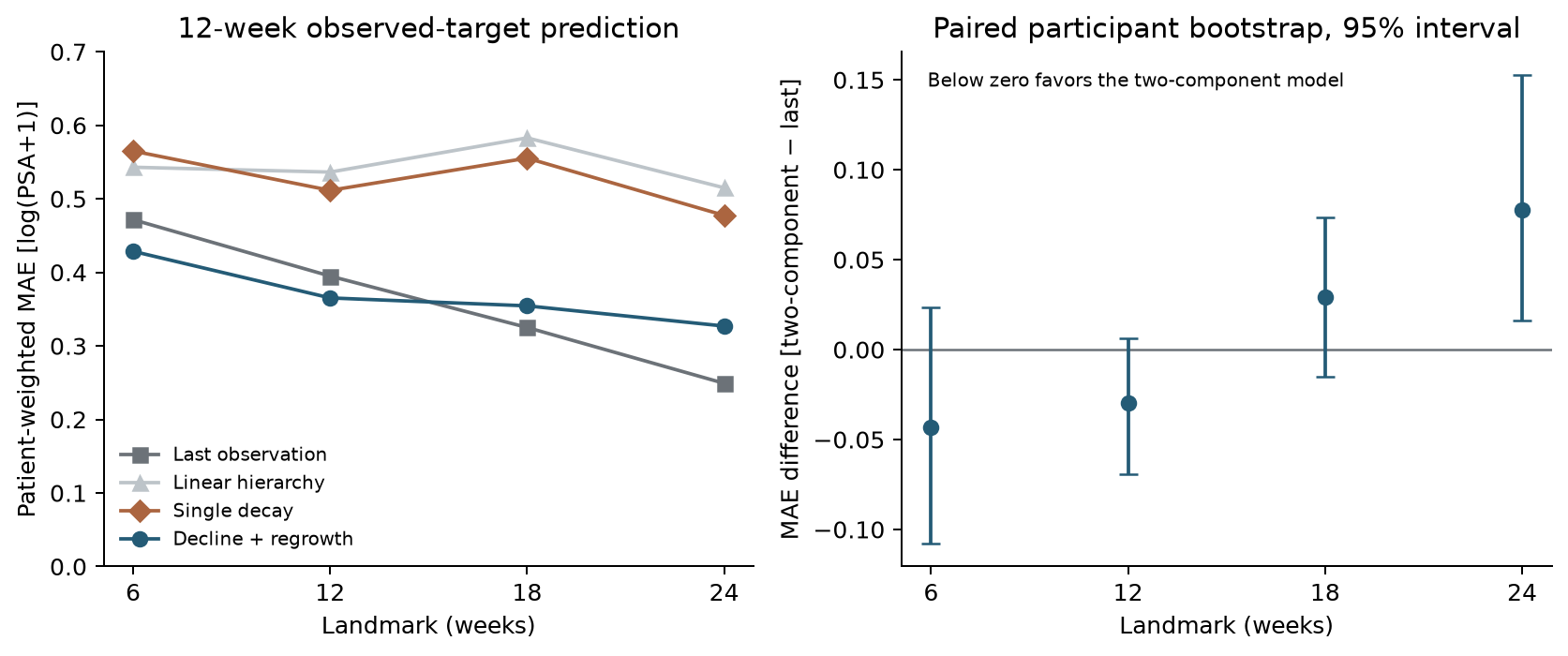
Figure 2. Left: point estimates on each landmark's observed target set. Right: two-component minus last-value MAE with a paired, patient-resampling 95% interval. Negative differences favor the two-component candidate. The resampling is conditional on the fitted models, and the four landmarks are not independent confirmatory tests.
| Landmark | Two-component − last MAE | Paired bootstrap 95% interval |
|---|---|---|
| 6 weeks | -0.043 | [-0.108, +0.024] |
| 12 weeks | -0.030 | [-0.070, +0.006] |
| 18 weeks | +0.029 | [-0.015, +0.074] |
| 24 weeks | +0.078 | [+0.016, +0.153] |
The two-component model's smaller error than the declining candidates is consistent with its ability to flatten as the declining component becomes small. However, the fitted regrowth component is nearly flat. Calling the improvement proof of detected regrowth would confuse flexibility with mechanism identification.
The differences from the last-value benchmark at 6 and 12 weeks are small and their resampling intervals cross zero. At 24 weeks, the two-component candidate is worse on this paired held-out comparison. No parameter or prior was selected using these test errors. The results do not justify discarding the simple benchmark or choosing a universal optimal observation duration.
Calibration is not the same as a narrow interval
| Landmark | Calibration patients | Two-component patient coverage | Full width | Last-value patient coverage |
|---|---|---|---|---|
| 6 weeks | 59 | 95.7% | 3.483 | 97.1% |
| 12 weeks | 67 | 98.6% | 2.988 | 98.6% |
| 18 weeks | 57 | 90.6% | 2.121 | 98.1% |
| 24 weeks | 45 | 88.4% | 1.496 | 95.3% |
Full width is on the supplied transformed scale. The nominal patient-level target is 90%, and coverage is evaluated over all observed on-treatment targets per patient in the 12-week window.
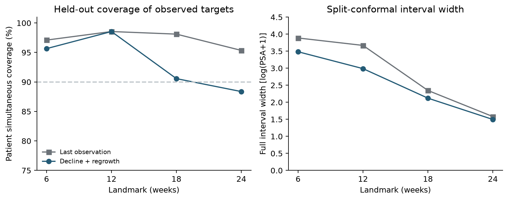
Figure 3. A separate calibration set adjusts the interval radius; the test set assesses it. High early coverage comes with broad intervals. At 24 weeks the two-component candidate covers 88.4% of test patients, compared with 95.3% for the last-value predictor. These finite-test estimates have sampling uncertainty; neither number establishes clinical acceptability.
For scale, a radius of 1.742 at 6 weeks means a roughly 5.7-fold factor on PSA+1, not a precise prediction. Coverage alone would conceal that lack of resolution. These calibrated prediction intervals are not confidence intervals for \(g\) or tumor biology.
Identification: the prior must not supply the conclusion
| Landmark | Eligible test patients | Data rank <4 | Data condition >10⁶ | Median g SD ratio |
|---|---|---|---|---|
| 6 weeks | 70 | 70 | 70 | 0.999999 |
| 12 weeks | 72 | 18 | 72 | 1.000000 |
| 18 weeks | 61 | 1 | 61 | 0.999989 |
| 24 weeks | 48 | 0 | 46 | 0.999966 |
The SD ratio is the local conditional standard deviation of log regrowth rate divided by its fitted prior SD. It is based on an uncensored Gauss–Newton approximation and is a diagnostic, not a qualified posterior interval.
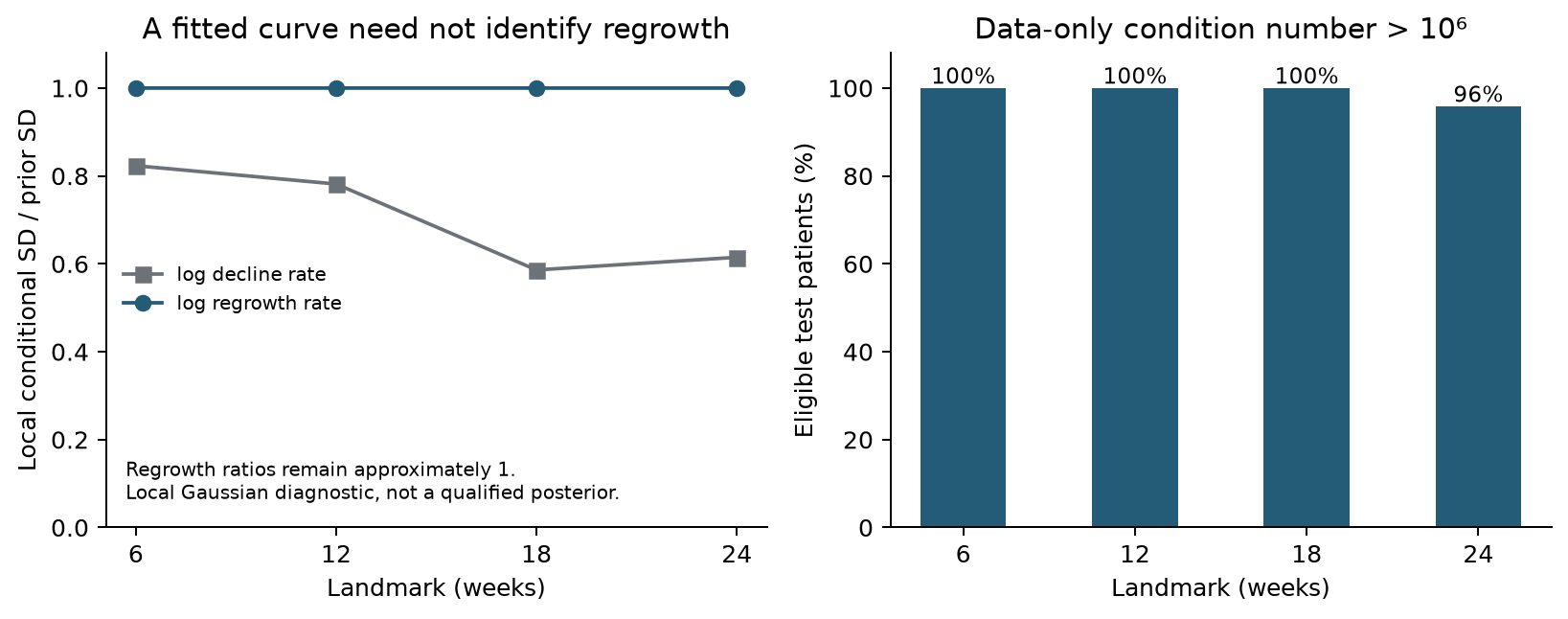
Figure 4. Regrowth SD ratios remain approximately one. The data-only information matrix is singular or ill-conditioned for most eligible test patients. Its rank improves with more observations, but full algebraic rank alone does not mean a reliable rate estimate.
Every two-component population fit places mean log regrowth at the specified lower bound, \(-10\). Most individual fits also have a bound-active parameter. All population starts report convergence and closely agreeing objectives, but numerical convergence does not turn a bound-active estimate into an identifiable biological quantity. At 6 weeks all 70 eligible test patients have data-only rank below four; even at 24 weeks 46 of 48 have condition number above \(10^6\).
I therefore do not publish individually definitive growth/decline estimates or convert these parameters into treatment recommendations. The supported statement concerns this bounded model and this first-order estimator. It does not establish that regrowth is unidentifiable under every likelihood, a richer mechanistic model, a longer complete series, or a fully joint analysis.
Sensitivity: shrinkage and treatment boundaries matter
| Landmark | Prior SD ×0.5 | Primary | Prior SD ×2 | Including post-treatment targets |
|---|---|---|---|---|
| 6 weeks | 0.504 | 0.429 | 0.388 | 0.451 |
| 12 weeks | 0.392 | 0.365 | 0.359 | 0.399 |
| 18 weeks | 0.380 | 0.354 | 0.345 | 0.361 |
| 24 weeks | 0.361 | 0.327 | 0.301 | 0.392 |
The prior-scale columns use the same primary target patients; the post-treatment column changes the target set and is not a paired treatment-effect comparison.
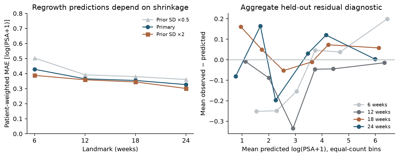
Figure 5. Left: changing individual prior SD changes predictions without changing the population fit. Right: mean residuals in equal-count prediction bins expose remaining errors. Only aggregate bins are shown; no participant trajectories or IDs are published.
Doubling individual prior SD reduces two-component MAE at 6 weeks from 0.429 to 0.388; halving it increases MAE to 0.504. This is evidence of sensitivity, not permission to choose the doubled prior after viewing the test set. At 24 weeks the observed post-treatment sensitivity has MAE 0.392 across 44 patients, compared with 0.327 across 43 patients in the primary target. Extrapolation across treatment cessation changes the interpretation and availability.
Omitting individual BLQ history gives the same main test errors here because test patients contributing the main prediction errors have no BLQ in their landmark histories. This statement does not include eligible patients without observed prediction targets. That sensitivity is uninformative about handling BLQ in general. Future BLQ targets are excluded from the main errors, and uncensored-only population fitting remains a limitation. A 42-day forecast-window analysis is also included in the companion with its own target counts.
What can be decided?
This analysis supports keeping the latest-value predictor as a serious benchmark, separating predictive accuracy from regrowth identification, and auditing risk-set changes before interpreting improvement with time. It also shows the exact conditions under which this implemented hierarchy adds little or loses predictive performance.
It does not establish a minimum observation period for a regrowth-based treatment decision. None of the examined windows resolves the identified rate-estimation problem under this estimator, and landmark comparisons involve different selected patients. Nor does it evaluate a future trial's benefit–risk or prove PSA surrogacy for survival.
For a new development program, the practical sequence is to specify the decision and target population, preserve treatment/measurement timing, include a last-value comparator, use a full censored nonlinear estimator if parameters will drive decisions, and then require prospectively specified validation of both prediction and decision performance. The present result cannot be transferred as a validated cutoff to another therapy.
Limits and reproducibility
This is one publicly distributed treatment-group subset with internal validation. It lacks the original independent validation patients, detailed dose histories and treatment-switch causes. Treatment cessation, death and measurement availability create selection that is not solved by splitting patients or adding a conformal interval. Missing-not-at-random behavior is not identified. Small later test groups and the fixed split limit precision.
The first-order population approximation, diagonal random-effects hierarchy, numerical bounds, partly omitted censoring likelihood and local information approximation are substantial methodological limits. Their effect on apparent regrowth cannot be separated completely here. A full nonlinear/joint model and genuinely independent cohort would be needed for stronger parameter and clinical claims. No such completed analysis is implied.
The companion contains the acquisition/hash check, transformation and audit code, fixed protocol, model implementation, aggregate results, five original figures, verification tests and an executed notebook. Raw data and individual parameters are not redistributed. The notebook reruns the analysis from the official download. All tables are generated from the saved results rather than manually transcribed.
References
- Desmée S, Mentré F, Veyrat-Follet C, Sébastien B, Guedj J. Using the SAEM algorithm for mechanistic joint models characterizing the relationship between nonlinear PSA kinetics and survival in prostate cancer patients. Biometrics. 2017;73:305–312. DOI, open author manuscript. Data provenance and observation definition; the present estimator differs.
- MonolixSuite documentation. PSA and survival data set. Public CSV accessed 2026-10-04; recorded SHA256 in companion.
- Angelopoulos AN, Bates S. A Gentle Introduction to Conformal Prediction and Distribution-Free Uncertainty Quantification. arXiv:2107.07511. Background for finite-sample split calibration; selection assumptions remain necessary here.
Download original code, aggregate results and executed notebook
Cite this article
Kumakura, D. (2026). Does separating PSA decline and regrowth improve early prediction?. daikikumakura.github.io. https://daikikumakura.github.io/writing/psa-early-observation.html