Cancer cachexia episodes and the prediction clock
A cachexia episode-table audit, checked against the paper's text and code, distinguishes retrospective interval starts, nadir, and end, and shows why its blood analyses and risk models do not test lead time.
On this page
“A blood signal appears before weight loss” sounds useful for early intervention. But “before” depends on the clock: the last stable measurement, first crossing of a loss threshold, and retrospectively identified start of a loss interval are different dates.
Castillon and colleagues' cancer-cachexia atlas treats weight loss as potentially recurrent episodes in records from 52,236 patients. It was published on October 12, 2026 (1).
I read the open-access paper (including Methods, Results, and Discussion), the released episode table and data dictionary, the detection code at a pinned commit, and some of the figure scripts. I did not check the Supplementary Tables, Extended Data, individual-level laboratory data, or the intermediate files that the figure scripts load. The released table contains no longitudinal blood measurements, so rather than claiming to predict a prodrome, I first established what the weight-loss clock means. There are two questions. What do the time variables in the released table mean? And what does that meaning leave for reading the paper's blood analyses and prediction models?
One cachexia label per patient is insufficient
The paper links 1,741,505 longitudinal body mass index (BMI) measurements with laboratory and tumor information in adults who underwent MSK-IMPACT (the Memorial Sloan Kettering tumor gene-panel test). From the 79,240 patients for whom data were obtained, it excludes patients with multiple primary cancers, a diagnosis date after the first BMI measurement, age under 18 years, no BMI data, fewer than two BMI measurements, or less than 180 days of BMI follow-up. Eligibility therefore requires adequate weight records and follow-up; this is not an unselected population of all cancer patients (original Methods, 1).
The basic criterion is at least 5% loss within 180 days, or at least 2% when starting smoothed BMI is below 20. The paper presents this as based on the international consensus criteria of Fearon et al. (weight loss above 5%, or above 2% with BMI below 20 kg/m² or sarcopenia) (2). BMI is smoothed with an exponentially weighted moving average (α = 0.2), and the criteria are applied to the smoothed trajectory. Overlapping candidate intervals are merged, and only those lasting at least 15 days are retained. Quality control removes intervals that overlap an edema-like window, defined as a gain of at least 5% that returns to within 2% within 30 days, because such transient gains can create spurious losses (1).
These are weight-defined episodes. The consensus definition also involves loss of muscle mass, incomplete reversal by conventional nutritional support, and functional impairment, but the paper reports as limitations that muscle imaging and nutrition-support records were not available across the full cohort and these elements could not be implemented (1, 2). An episode ending does not mean the underlying syndrome is cured.
The public CSV and dictionary contain 58,817 rows (3). Patients with episodes may have multiple rows; patients without an episode have one nonepisode row.
Table 1. Patients and intervals in the public episode table.
| Aggregate | Result |
|---|---|
| Unique patients | 52,236 |
| Patients with episodes | 24,357 (46.63%) |
| Episodes | 30,938 |
| Patients with at least 2 episodes | 5,496 |
| Fraction with at least 2 episodes among affected patients | 22.56% |
Patient proportions count each person once. Episode-duration summaries instead count intervals, not patient-average durations. Treating 30,938 episodes as that many patients would repeatedly count recurrent cases.
This aggregation agreed with the paper's text: 46.63% of patients had episodes and 22.56% of affected patients had multiple episodes, and, from the patient flags for the 10% and 15% criteria, 19.4% and 6.9% of patients (1). Because the values come from the same table, this is not independent validation; it confirms only that the released table corresponds to the paper's detection results (calculation: results/summary.json).
The code separates interval start from threshold crossing
The dictionary defines start_day as the reference time at which the detection window is triggered (the baseline of the 180-day sliding window). end_day is the last day at which the merged interval still meets the criterion, not the nadir. The pinned detection README explicitly searches forward from each reference day (4). In the script at that commit, each measurement day serves as a baseline; the first day within the following 180 days on which smoothed BMI is lower than baseline by the threshold is recorded as onset_day, and the last such day as end_day; overlapping detections are merged. start_day is the earliest baseline day of the merged interval, so for the first detection onset_day can be as much as 180 days after start_day.
The paper's Methods describe episode start as the first qualifying timepoint (1). Read alone, this sentence could describe something close to onset_day. For columns of the released table, this article follows the dictionary and code and treats start_day as the baseline day. The difference from the paper's wording remains unresolved.
Looking ahead is legitimate when defining retrospective intervals. Interpreting the reference day as the day when cachexia could already have been detected changes the use. Consider an illustrative record, not an actual patient:
Table 2. Hypothetical weights illustrating information available on each day.
| Day | Weight | Information available by then |
|---|---|---|
| 0 | 70.0 kg | Candidate reference measurement |
| 30 | 69.0 kg | From day 0, approximately 1.4% loss |
| 90 | 66.0 kg | From day 0, approximately 5.7% loss |
Using raw measurements in this simple example, loss of at least 5% from day 0 becomes known on day 90. The three-point example does not reproduce the original smoothing and merging procedure. An exponentially weighted moving average with α = 0.2 retains past measurements, so a declining series can reach the criterion later after smoothing. The public code uses pandas' default normalization (adjust=True); in a finite series the latest measurement does not always have weight 0.2. The released episode table lacks onset_day: it contains start, nadir, and end, but cannot reconstruct first threshold crossing. Start-to-nadir duration therefore cannot be called detection delay or an intervention window.
A 180-day detection window can produce longer episodes
Among 30,938 episodes, median start-to-nadir duration is 196 days, with interquartile range 147–273; median start-to-end duration is 212 days. This is compatible with a 180-day search window because overlapping candidates merge into longer intervals.
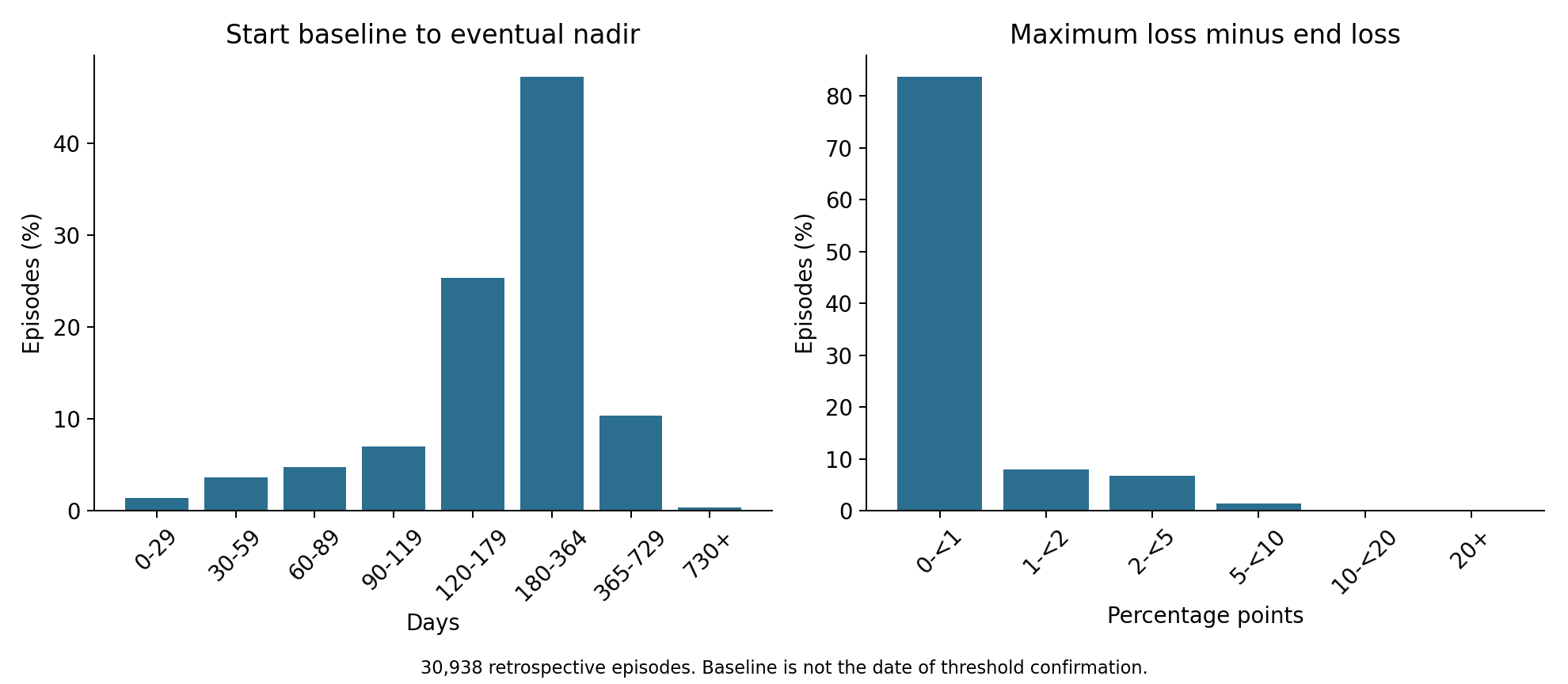
Figure 1. Author's calculation from the public episode table: left, reference-day to minimum-BMI duration; right, maximum minus end-of-interval percentage loss. These retrospective quantities do not measure prospective detection time or intervention opportunity.
In 11,685 intervals, or 37.77%, maximum loss exceeds end-of-interval loss: the nadir precedes the end, and BMI at the end is higher than at the nadir. Weight can partially recover while merged candidate windows still meet criteria, so end need not coincide with the minimum. The interval from nadir to end had a median of 0 days, a 75th percentile of 28 days, a 90th percentile of 67 days, and a maximum of 363 days.
End weight defines a different event
All 30,938 maximum-loss values meet their applicable thresholds. Using start-to-end loss alone instead places 1,376 episodes, 4.45%, below threshold.
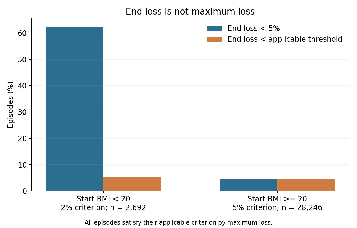
Figure 2. Author's comparison of two released summary values, retaining the 2% threshold below starting BMI 20 and 5% otherwise. It does not rerun episode detection.
Table 3. Starting-BMI-specific thresholds and end-of-interval classifications.
| Starting smoothed BMI | Applicable loss threshold | Episodes | End loss below applicable threshold |
|---|---|---|---|
| Below 20 | 2% | 2,692 | 140 |
| At least 20 | 5% | 28,246 | 1,236 |
Applying only “end loss below 5%” yields 2,915 intervals, including those originally assigned the 2% criterion. That would overstate missed episodes. This discrepancy does not establish an algorithmic defect: maximum loss within an interval and its final state describe different quantities. According to the dictionary, end_day is the last day that meets the criterion relative to some baseline within the interval, which is not necessarily the start_day baseline, so loss measured from start_day need not meet the criterion at end_day.
The choice of summary value changes few intervals. The difference between maximum and end-of-interval loss was 0 in 62.23% of intervals, 1.7 percentage points at the 90th percentile, and at most 19.6 percentage points. A difference of 5 percentage points or more occurred in 468 intervals (1.51%). In the text I read, the paper does not state which loss underlies its mean weight loss of 10.45% or its weight-loss grading system (WLGS) grades (1). The two quantities coincide for most intervals, but for severity at the interval level the choice can change the result in those 468.
One row ends beyond its recorded observation/survival duration. I retained all rows in the main descriptive summary and checked exclusion sensitivity without inventing a corrected date or using the row for survival analysis. Details are recorded in the distributed archive.
Blood associations differ from predicting future loss
The paper examines blood features during episodes and tumor-genomic associations. The blood analysis is a mixed-effects logistic regression with episode status as the outcome, the laboratory value, age, and sex as predictors, and a random intercept per patient; a laboratory test is classified as inside or outside an episode by whether its date overlaps the episode interval (1). The mean log2 odds ratio for albumin was −0.89 (95% confidence interval −1.01 to −0.76), and subnormal values occurred in 28.4% of measurements within episodes versus 12.0% outside. The authors themselves describe the changes as modest, largely within reference ranges, and note that some markers could reflect concurrent chemotherapy rather than cachexia (1).
A difference in laboratory values during episodes is thus a description of concurrent states. Anticipating future loss requires a separate validation.
The paper's risk models do not use blood values as inputs. They are Cox-regression nomograms based on stage, ECOG–KPS, baseline BMI, and mutations such as TP53 and STK11, and they address cumulative episode probability at one, two, and three years after diagnosis. The C-indices were 0.648 for lung adenocarcinoma, 0.670 for prostate, and 0.639 for colorectal cancer. The Methods describe 200 bootstrap resamples of each full cancer-specific cohort for their intervals; these differ from calibration and time-dependent AUC evaluated on the 50% held-out subset; for external (DFCI) evaluation, a reduced model restricted to shared variables was tested in lung cancer because ECOG–KPS was unavailable, with a C-index of 0.625 (1). That differs from sequential blood-based forecasting of imminent loss. I neither retrain those models nor test blood-signal lead times. The paper does not claim blood-signal lead time either.
What does the ambiguity of the interval clock leave for reading these results? The paper describes its time-dependent survival models as switching episode status from 0 to 1 at the onset of the first episode, and classifies blood tests by overlap with episode intervals (1). In the pinned commit, the figure script for the survival analysis renames the columns start_day and end_day of an interval file as the start and end of the exposure interval. I could not check how that file was built, so from what I read I cannot determine whether the published hazard ratios and blood comparisons are anchored on start_day or on onset_day.
If start_day is the interval start, the reading changes as follows. The “exposed” period of a time-dependent model begins up to 180 days before threshold attainment could be observed. Patients in that period are, by definition, those who survived and remained under observation until they later met the criterion. Exposure defined by future survival is the structure of immortal time, which tends to make deaths in the exposed group look fewer (5, 6). The blood comparison “during episodes” would also include tests taken before the criterion was met. The comparison would then be neither a difference in states after threshold crossing nor a prodrome, but a mixture of the two. The direction and size of the effect cannot be estimated from the released table and the sources I read. Whether this structure occurs in the published analysis remains unconfirmed. I do not assign a direction or magnitude of bias to the published hazard ratios; establishing the interval-file provenance and time origin comes first.
As related work, Yin et al. reported a machine-learning model that predicts, from weight changes up to admission, potentially reversible cachexia (a cachexia diagnosis at baseline that turned negative one month later), and Chen et al. reported models that identify precachexia and cachexia from baseline characteristics, including HDL and the C-reactive protein–albumin ratio (7, 8). I checked only the abstracts of these two studies, so I do not assess their methods or validation design. Both address classification at a point in time or short-term prediction, whereas the paper concerns the timing of episodes in a health-system record, so the questions differ. Still, the condition that a prediction may use only information available by that day applies to any design.
Future nadir and interval end are unavailable before the interval ends. Information allowed in retrospective labels differs from information available to a predictor on a particular day. An unmeasured blood value is not a normal one, and an absence of weight records does not show that loss stopped. Observation frequency and censoring can mix biological change with changes in opportunities for clinical recording. Even 30,938 episodes do not resolve what was known on each day.
Conclusion
Testing “a blood signal appears before weight loss” requires distinguishing the prediction date from the threshold-crossing date and using only tests available by the prediction date. If lead time is measured relative to threshold crossing, that crossing must be ascertainable from information available by that day. The released episode table does not have that day (onset_day). start_day is a reference day chosen by looking 180 days ahead, and nadir_day and end_day are likewise determined retrospectively. This table therefore cannot yield a lead time for a signal or an opportunity for intervention.
What could be established is the following. Of 52,236 patients, 24,357 (46.63%) had 30,938 episodes, and the intervals last a median of 212 days, beyond the 180-day detection window. In 37.77% of intervals the BMI at the end is higher than at the nadir, and judging by end weight alone would place 1,376 episodes (4.45%) below their criterion. The paper's blood analysis describes concurrent differences, and its risk prediction does not use blood as input. Whether blood signals precede weight loss has not been tested, either in the paper or here.
This article's checks are a clarification of definitions based on the released table, dictionary, and code, not a reanalysis on individual-level data or intermediate files. I found no evidence that reverses the direction of the paper's main results.
Data and code availability
The code, aggregate inputs, outputs, and figures document denominators, thresholds, durations, and exclusion sensitivity. Patient identifiers and individual episode records are excluded; acquisition/aggregation scripts and sources are provided. Original figures and implementation are not redistributed.
python -m pip install -r requirements.txt
python analysis.py
python -m unittest test_analysis.py
python plot.py
The additional aggregation script reproduces the added gap counts and quantiles. With pandas installed and the cited public CSV downloaded, run python extra-episode-checks.py path/to/table.csv. It prints no patient identifiers or individual rows.
Sources were checked on October 18, 2026 for the released table and code, and on October 29, 2026 for the paper's text: the original paper (1), the released table and dictionary (3), and the detection README and script at the pinned commit (4).
References
-
Castillon VJ, Xie AX, Boscenco S, Tse E, Ruthen N, Wang J, et al. A health-system-scale, episode-resolved multimodal atlas of cancer cachexia. Nat Med. 2026. doi:10.1038/s41591-026-04689-9. Published online 2026 Oct 12.
-
Fearon K, Strasser F, Anker SD, Bosaeus I, Bruera E, Fainsinger RL, et al. Definition and classification of cancer cachexia: an international consensus. Lancet Oncol. 2011;12(5):489–495. doi:10.1016/S1470-2045(10)70218-7.
-
Reznik E, Castillon VJ. A health-system-scale, episode-resolved multimodal atlas of cancer cachexia [dataset]. Zenodo. 2026. doi:10.5281/zenodo.22045313.
-
Reznik Laboratory. Cancer cachexia episode identification [source code]. Commit 5d63b83a7ca3915949d4a0131e8b0c7ec52f8903. Detection-code README.
-
Lévesque LE, Hanley JA, Kezouh A, Suissa S. Problem of immortal time bias in cohort studies: example using statins for preventing progression of diabetes. BMJ. 2010;340:b5087. doi:10.1136/bmj.b5087.
-
Suissa S. Immortal time bias in pharmaco-epidemiology. Am J Epidemiol. 2008;167(4):492–499. doi:10.1093/aje/kwm324.
-
Yin L, Li N, Lin X, Zhang L, Fan Y, Liu J, et al. Early identification of potentially reversible cancer cachexia using explainable machine learning driven by body weight dynamics: a multicenter cohort study. Am J Clin Nutr. 2025;121(3):535–547. doi:10.1016/j.ajcnut.2025.01.006.
-
Chen Y, Liu C, Zheng X, Liu T, Xie H, Lin SQ, et al. Machine learning to identify precachexia and cachexia: a multicenter, retrospective cohort study. Support Care Cancer. 2024;32(10):630. doi:10.1007/s00520-024-08833-4.