Zongertinib weight-based dosing and exposure distributions
Public PopPK and FDA model-derived ratios compare fixed, weight-band and theoretical continuous dosing. Conditional simulations separate boundary discontinuities from residual variability without predicting clinical benefit.
On this page
- Background and objective
- Background to the 90 kg boundary
- Recovering the dose-comparison table's equation
- Three dose designs
- Individual variability remains after weight adjustment
- A mathematical switching point near 90 kg
- Auxiliary concentration reconstruction
- Discussion
- Numerical checks and limitations
- Data and code availability
- References
Background and objective
US zongertinib dosing is 120 mg once daily below 90 kg and 180 mg once daily at 90 kg or above. The regimen accounts for weight but does not make everyone's exposure identical.
Using public PopPK coefficients and FDA dose-comparison tables, I calculated what this adjustment changes. Fixed 120 mg dosing yields decreasing AUC with increasing weight; the two-band regimen offsets that decline at higher weights but retains a dose step at 90 kg. A theoretical continuous adjustment removes the weight trend without removing individual variability.
The objective is to identify what exposure matching equalizes and what remains. This is neither a new patient-data model fit nor a proposal to change the approved regimen.
Background to the 90 kg boundary
Zongertinib is an oral inhibitor for non-squamous non-small cell lung cancer with HER2, ERBB2, TKD activating mutations. Initial US approval was in 2025, followed by an indication expansion in February 2026. The July 2026 label revision retains the 120/180 mg weight-based regimen (1, 2).
The original FDA review considered ORR at low exposure, lower exposure among heavier patients, matching exposure with 180 mg and benefit–risk when selecting 90 kg. The calculations below do not replace that clinical assessment (3, PDF pp. 358 and 361).
Table 1. Question and comparison conditions.
| Item | Definition |
|---|---|
| Question | How do fixed dosing, two bands at 90 kg and continuous weight adjustment change steady-state AUC distributions and concentrations near the boundary? |
| Intended use | Audit of exposure design using a public model; not individual prescribing or trial-dose selection |
| Reference | Typical-individual AUC at 70 kg and 120 mg QD, every 24 hours |
| Common conditions | Age, race and formulation effects fixed; interoccasion variability, IOV, and measurement error excluded |
| Virtual individuals | 4096 per weight stratum, sharing random effects across dose designs; no patient weight-frequency distribution assumed |
Recovering the dose-comparison table's equation
The public PopPK model combines sequential zero-order input and first-order absorption with two-compartment distribution. Key coefficients are listed below (3, Table 79, PDF pp. 297–298).
Table 2. Published PopPK coefficients used in the reconstruction.
| Quantity | Published value | Treatment in this calculation |
|---|---|---|
| CL/F | 7.22 L/h | Fixed-effect coefficient |
| Vc/F, Vp/F | 82.6, 48.2 L | Fixed-effect coefficients |
| Q/F | 3.55 L/h | Fixed-effect coefficient |
| Zero-order duration D1, first-order ka | 1.03 h, 1.22 h⁻¹ | Auxiliary concentration reconstruction |
| MAT, MATfr | 1.85 h, 0.443 | Published absorption parameters; variability implementation described below |
| Weight exponent for CL and Q | 0.75 | Fixed in the original model |
| Weight exponent for Vc and Vp | 1.0 | Fixed in the original model |
| IIV CV for CL, Vc and MAT | 0.244, 0.285, 0.415 | Converted from CV to log variance |
| CL–Vc correlation | 0.601 | Retained in virtual-individual generation |
With common formulation and background conditions, daily steady-state AUC is:
\[ AUC_{0-24,ss}(w,D)=\frac{D}{CL_{70}(w/70)^{0.75}}. \]
Its ratio to the 70 kg, 120 mg reference is:
\[ r(w,D)=\frac{AUC(w,D)}{AUC(70,120)} =\frac{D}{120}\left(\frac{w}{70}\right)^{-0.75}. \]
Common reference clearance, formulation F and absorption rate cancel. The main AUC question can therefore be handled by this simple equation. The covariate comparison in FDA Figure 19 uses 70 kg, age 62, non-Asian background and SDD or SDD iCF formulation as reference conditions. Common background effects cancel in these AUC ratios. For the auxiliary profiles below, those covariate multipliers are suppressed to 1 and CL/F=7.22 is used as the 70 kg reference coefficient. The profiles do not reproduce all background adjustments underlying the source's absolute concentrations.
FDA Table 89 gives 13 integer-percentage ratios for 120 mg across 33.6–122 kg and eight for 180 mg across 75–122 kg. Fitting only the 120 mg rows by least squares to:
\[ \log r_k=-a\log(w_k/70) \]
gave \(a=0.74796\). The maximum difference from the 120 mg table was 0.495 percentage points; the held-out 180 mg table differed by at most 0.456 points (3, Table 89, PDF p. 361).
This reverses a rounded model-derived table. It does not newly estimate an allometric exponent from clinical data. Checking the 180 mg rows is internal numerical auditing of the same model, not external validation. Subsequent analyses use the published fixed exponent of 0.75, without a clinical confidence interval for the recovered coefficient.
Three dose designs
\[ D_{fixed}(w)=120, \]
\[ D_{step}(w)= \begin{cases} 120 & w<90,\\ 180 & w\ge90, \end{cases} \]
\[ D_{continuous}(w)=120\left(\frac{w}{70}\right)^{0.75}. \]
The third design is a mathematical comparator canceling the assumed weight-related AUC trend. It is not approved dosing. At 90 kg it gives 144.9 mg, which cannot be administered directly as an integer number of current 60 mg tablets. It proposes neither lower doses in lighter patients nor higher doses in heavier patients.
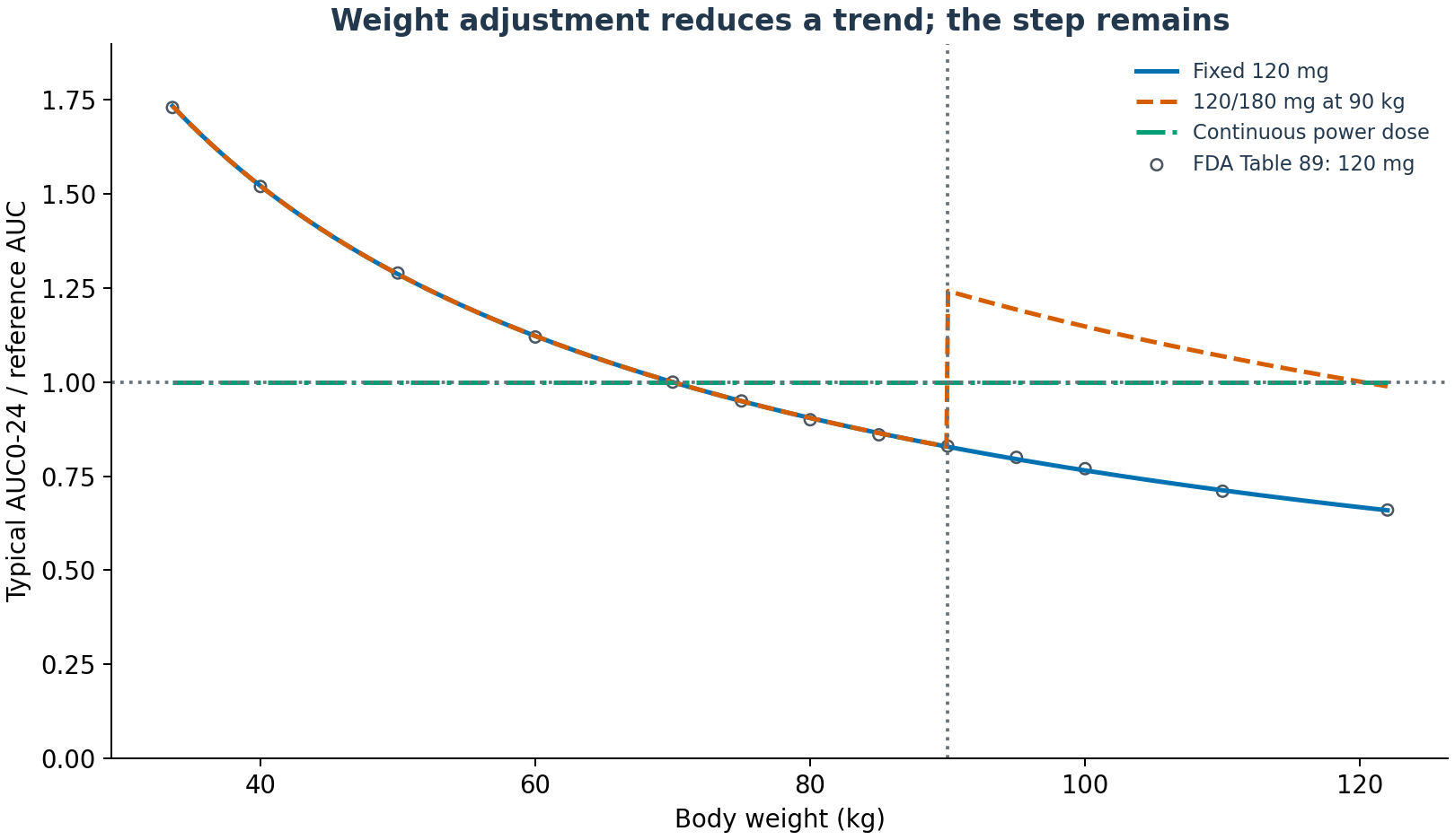
Figure 1. The reference is the typical 70 kg individual receiving 120 mg. Open points are FDA model-table values, not measured AUCs. Lines are calculated here; the discontinuity comes from the dose rule.
Table 3. Typical-individual AUC ratios by weight and design.
| Weight | Fixed 120 mg | Two-band regimen | Continuous adjustment |
|---|---|---|---|
| 70 kg | 1.000 | 1.000 | 1.000 |
| 89.9 kg | 0.829 | 0.829 | 1.000 |
| 90 kg | 0.828 | 1.242 | 1.000 |
| 110 kg | 0.712 | 1.069 | 1.000 |
The two-band regimen offsets lower exposure at 110 kg. Between 89.9 and 90 kg, however, the change from 120 to 180 mg increases the AUC ratio approximately 1.499-fold despite little weight difference. These are separate steady-state conditions. The analysis does not validate an immediate dose-change rule following a transient 0.1 kg fluctuation in one patient.
Continuous adjustment gives ratio 1 by construction because dose and clearance share the same weight exponent. This is not a newly discovered drug effect.
Individual variability remains after weight adjustment
For virtual individuals:
\[ CL_i=CL_{70}\left(\frac{w}{70}\right)^{0.75}e^{\eta_{CL,i}}, \quad \eta_{CL,i}\sim N(0,\omega_{CL}), \]
\[ \omega_{CL}=\log(1+0.244^2) \]
The reported CV is not substituted directly as log variance.
The same 4096 random-effect sets are used at each weight and across all designs. Because no joint patient weight-frequency distribution is reconstructed, I do not calculate an overall patient-average exposure or proportion improved.
For illustration, I count exposure below 0.8 and above 1.25 times the typical reference AUC. These cutoffs are neither a therapeutic window, efficacy or toxicity thresholds, nor a bioequivalence criterion. They are descriptive scale markers.
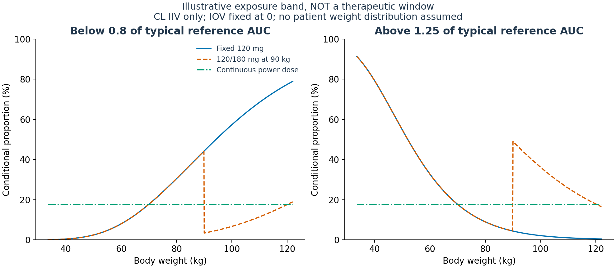
Figure 2. Theoretical proportions from the log-normal CL IIV distribution, calculated analytically as smooth curves separately from the main 4096-individual simulation. IOV is 0. The curves represent neither all-patient prevalence nor clinical risk.
Table 4. Conditional AUC distributions from 4096 virtual individuals.
| Weight and design | Median AUC ratio [5th–95th percentile] | Below 0.8 | Above 1.25 |
|---|---|---|---|
| 70 kg, 120 mg | 1.001 [0.673–1.492] | 17.8% | 17.4% |
| 89.9 kg, two bands | 0.830 [0.558–1.237] | 43.8% | 4.6% |
| 90 kg, two bands | 1.244 [0.836–1.854] | 3.5% | 49.2% |
| 110 kg, fixed 120 mg | 0.713 [0.480–1.063] | 67.9% | 0.9% |
| 110 kg, two bands | 1.070 [0.720–1.595] | 11.3% | 26.1% |
| 110 kg, continuous | 1.001 [0.673–1.492] | 17.8% | 17.4% |
Even continuous adjustment retains an approximately 0.67–1.49 percentile range, because removing weight's contribution does not remove within-weight clearance variability. These are percentiles across virtual individuals, not confidence intervals for estimates.
The original model includes IOV in MAT and in relative F with a Box–Cox transformation. Without the original executable implementation, I did not replace those components with arbitrary normal draws; both IOV effects were fixed to 0. These distributions therefore exclude some clinical variability across individuals, occasions and backgrounds.
A mathematical switching point near 90 kg
Consider choosing between 120 and 180 mg to minimize the absolute log-distance from the reference AUC:
\[ D^*(w)=\arg\min_{D\in\{120,180\}}|\log r(w,D)|. \]
Equal log-distances at the switching point give:
\[ w^*=70\times1.5^{1/(2a)}. \]
For \(a=0.75\), the boundary is 91.7 kg. Its proximity to 90 kg does not reproduce FDA's decision function. It follows from my chosen 70 kg reference, two candidate doses and log-distance objective, without efficacy, safety or formulation considerations.
Assumed exponents of 0.5, 0.75 and 1.0 give switching weights of 105.0, 91.7 and 85.7 kg. Because the original model fixes 0.75, adding more rounded table values cannot independently validate that structural assumption. This range is not an estimated confidence interval for the exponent.
Auxiliary concentration reconstruction
For concentration profiles, zero-order input enters an absorption compartment followed by first-order absorption and two-compartment disposition:
\[ \frac{dA_g}{dt}=u(t)-k_aA_g,\qquad u(t)=\begin{cases}D/D_1 & 0\le t<D_1,\\0 & D_1\le t<24,\end{cases} \]
\[ \frac{dA_c}{dt}=k_aA_g-\frac{CL+Q}{V_c}A_c+\frac{Q}{V_p}A_p, \quad \frac{dA_p}{dt}=\frac{Q}{V_c}A_c-\frac{Q}{V_p}A_p, \quad C=\frac{A_c}{V_c}. \]
CL and Q scale with weight to the power 0.75, and both volumes to the power 1. The table supplies reference apparent coefficients. Because CL/F and other apparent terms are used, the absolute bioavailability of 0.76 is not multiplied into the dose again. MAT variability is reconstructed by multiplying D1 and inversely scaling ka by the same factor.
There is an unresolved absorption-time discrepancy. First-order absorption proceeds while zero-order input continues, giving an input first moment of \(D_1/2+1/k_a=1.335\) h. The reported MAT is 1.85 h, numerically close to \(D_1+1/k_a\). Without the executable model or its naming conventions, I do not equate these quantities. Figure 3 is an auxiliary reconstruction, not a validated reproduction of the original absorption profile. Main AUC conclusions do not depend on this discrepancy; peak magnitudes and timing do.
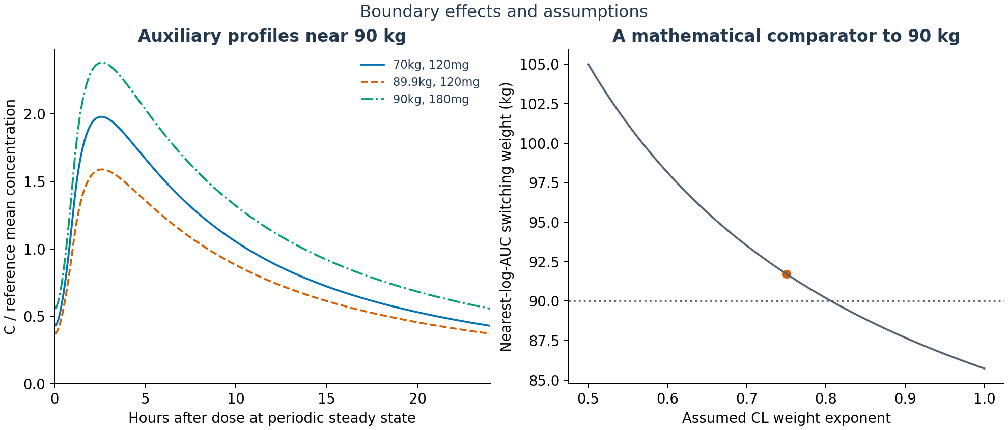
Figure 3. Left: auxiliary profiles with zero random effects, normalized to the 70 kg, 120 mg mean concentration. The absorption-moment discrepancy remains unresolved. Right: switching weight minimizing log-AUC distance, not a proposed approved-regimen change.
The calculated reference AUC was 31.0 µmol·h/L and Cmax 2.56 µmol/L, compared with label population geometric means of 34 and 3.0. Differences in reference covariates, aggregation over patients and occasions, and absorption implementation prevent interpreting this comparison as independent external validation (4, Section 12.3).
Discussion
The FDA review describes a positive exposure–ORR trend, without the same relationship established for every endpoint, including DOR and PFS. It cautions about interpretation at exposure extremes (3, PDF pp. 317, 358 and 361).
I do not insert these AUC predictions into existing E–R models to claim superior continuous dosing or insufficient efficacy just below 90 kg. The descriptive 0.8/1.25 cutoffs cannot be translated directly into response or adverse-event risk.
IOV and the joint distribution of background characteristics, actual dosing histories and outcomes are absent. A smaller exposure trend across weights therefore does not establish a ranking of clinically preferable regimens.
Numerical checks and limitations
Inputs, source pages, code and tables are retained. analysis/run_analysis.py regenerates the table inversion, 4096-individual calculations per weight, sensitivity analyses and three figures. Run python -m unittest discover -s analysis -p "test_*.py" -q for checks.
Nine tests passed, including agreement with model-derived tables, boundary conditions including exactly 90 kg, the log-distance switching formula, dose proportionality, an independent ODE solution, CV conversion and correlation. The maximum relative difference between AUC integrated on a 0.05-hour grid and mass-balance AUC was 0.00019%. These are numerical checks, not validation of predictions in patients.
Outputs are in outputs/tables/, recovered coefficients in outputs/fit.json and verification values in outputs/verification.json. Individual measured data, the full NONMEM implementation and an IOV-inclusive patient distribution were not obtained. The distribution contains original code, transcribed numerical inputs and original figures rather than images from source documents.
Data and code availability
Download analysis code, inputs, tables and rerun instructions.
References
- US Food and Drug Administration. FDA grants accelerated approval to zongertinib for unresectable or metastatic non-squamous non-small cell lung cancer. 2026 Feb 26. Approval announcement.
- Boehringer Ingelheim Pharmaceuticals Inc. HERNEXEOS (zongertinib tablets): US prescribing information. Revised 2026 Jul. DailyMed. Section 2.2.
- US Food and Drug Administration. HERNEXEOS (zongertinib), NDA 219042: Multi-Discipline Review. 2025. Review PDF. Table 79, Figure 19 and Table 89; PDF pp. 297–298, 317, 358 and 361.
- Boehringer Ingelheim Pharmaceuticals Inc. HERNEXEOS (zongertinib tablets): US prescribing information. Revised 2026 Feb. FDA label PDF. Section 12.3.