Telisotuzumab vedotin initial dosing with public PK and exposure-response models
A reproducible PK and exposure–response comparison of fixed and initial lower doses of telisotuzumab vedotin.
On this page
- Scope of the calculation
- Three dosing conditions
- ADC concentration model
- Early reduction and later recovery of exposure
- Which exposure belongs in the exposure–response equation?
- The dose ranking depends on value judgments
- ADC and MMAE can move in opposite directions
- Initial lower dosing remains unresolved by this equation
- Data and code availability
- References
Starting an anticancer drug at a lower dose and returning to the usual dose later is an attractive way to separate early risk from later exposure. Calculating the concentration profile is one task; predicting the efficacy and safety of that sequence is another.
I compared fixed 1.9 mg/kg, fixed 1.6 mg/kg, and 1.6 mg/kg for the first two doses followed by 1.9 mg/kg, using published pharmacokinetic and exposure–response models for the c-Met-targeted antibody–drug conjugate (ADC) telisotuzumab vedotin. Initial dose reduction separated early from later exposure, but an exposure–response equation that takes only first-cycle exposure could not establish the long-term value of this strategy.
Sources were checked on October 21, 2026. Telisotuzumab vedotin received US accelerated approval in 2025 for previously treated nonsquamous NSCLC with high c-Met protein overexpression. The approved dose is 1.9 mg/kg every two weeks, capped at 190 mg for patients weighing at least 100 kg (1).
Scope of the calculation
The question is how fixed dose reduction and initial lower dosing change early and later ADC exposure, and how those exposures map onto the published efficacy and toxicity associations.
The calculation supports research comparisons of dosing conditions and measurements. It does not select doses for individual patients. It considers objective response rate (ORR) and grade 3 or higher peripheral neuropathy (PN), rather than a comprehensive benefit–risk model that includes mortality and other safety outcomes.
The 2026 paper reports PK and exposure–response analyses involving 304 patients. Numerical inputs here came from Tables 47, 48, 51 and 54 of the FDA review, which covers the same development program. I used published coefficients for this drug without fitting a new individual-level nonlinear mixed-effects model (2, 3).
Three dosing conditions
All conditions were simulated every two weeks for 84 days. A 30-minute infusion was used consistently as a hypothetical simulation condition; this does not reproduce every approved administration instruction or premedication. The reference body weight was 68.9 kg, and the 100 kg dose cap was implemented.
Table 1. Dosing conditions; the interval was two weeks throughout.
| Condition | Days 0 and 14 | Day 28 onward |
|---|---|---|
| Fixed 1.9 | 1.9 mg/kg | 1.9 mg/kg |
| Fixed 1.6 | 1.6 mg/kg | 1.6 mg/kg |
| Initial two doses at 1.6 | 1.6 mg/kg | 1.9 mg/kg |
The FDA review discusses prospective investigation of lower initial dosing followed by 1.9 mg/kg, but part of the proposed duration is redacted. The first-two-dose duration is my hypothetical condition, not a reconstruction of an FDA-specified regimen (3, p. 235).
ADC concentration model
The ADC follows a linear two-compartment model:
\[ \frac{dA_c}{dt}=R_{\mathrm{in}}(t)-\frac{CL+Q}{V_c}A_c+\frac{Q}{V_p}A_p, \] \[ \frac{dA_p}{dt}=\frac{Q}{V_c}A_c-\frac{Q}{V_p}A_p, \qquad C_{ADC}=\frac{A_c}{V_c}. \]
Time is in days, amounts in mg, and volumes in L. Concentrations in mg/L are numerically equal to µg/mL.
Table 2. ADC model inputs from Tables 47 and 48 of the FDA review (3).
| Parameter | Value |
|---|---|
| CL | 1.34 L/day |
| Vc | 3.44 L |
| Q | 1.21 L/day |
| Vp | 2.41 L |
| Log-scale interindividual variance of CL | 0.0946 |
| Log-scale interindividual variance of Vc | 0.0268 |
The last two entries are variances of log-scale random effects, not coefficients of variation themselves. They correspond to reported CVs of 31.5% and 16.5%. I generated 4096 paired random effects and reused each pair across all dosing conditions. Residual error and fixed-effect estimation uncertainty were not included.
Because I could not fully establish the covariate centering constants from the original code, I defined a mathematical reference using the published fixed coefficients. Albumin varies only as a ratio \(r\) to that reference:
\[ CL_i=1.34\,r^{-0.970}e^{\eta_{CL,i}},\qquad V_{c,i}=3.44\,r^{-0.464}e^{\eta_{V,i}}. \]
The ratios \(r=0.75,1,1.10\) are not converted to actual g/L. Other covariate multipliers are fixed at one, and the CL and Vc random effects are independent in this conditional population. It does not reproduce the joint distribution of weight, age, ancestry and disease characteristics in patients, or estimate a causal effect of changing albumin.
Early reduction and later recovery of exposure
At albumin ratio one, I calculated within-patient AUC ratios relative to fixed 1.9 mg/kg.
Table 3. Median within-patient AUC ratios relative to fixed 1.9.
| Window | Fixed 1.6 | Initial two doses at 1.6 |
|---|---|---|
| Day 0–14 | 0.8421 | 0.8421 |
| Day 0–28 | 0.8421 | 0.8421 |
| Day 56–84 | 0.8421 | 0.99997 |
| Day 0–84 | 0.8421 | 0.9468 |
These are medians across 4096 paired ratios. Linearity makes the fixed-1.6 ratio equal to 1.6/1.9 in every window. With the first two doses reduced, later exposure almost returned to the reference. The 5th–95th percentile range for the Day 56–84 ratio was 0.99948–1.00000. This describes variability among conditional virtual patients, not a confidence interval.
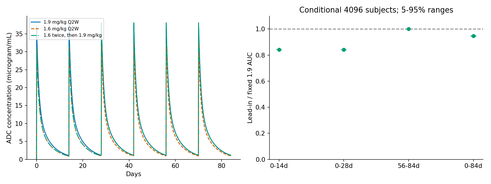
Figure 1. ADC concentration profiles and interval-specific AUC ratios calculated by the author.
Although the overall 84-day AUC reduction was about 5%, exposure during the first 28 days was about 16% lower. Total AUC alone hides this redistribution over time. These results assume a linear, time-invariant model; they do not capture changes in deconjugation or clearance as tumor burden changes.
Which exposure belongs in the exposure–response equation?
The paper reports separate regressions for several exposure metrics. I selected the equations using the mean ADC concentration during the first two weeks:
\[ E=C_{\mathrm{avg,C1}}=\frac{AUC_{0-14}}{14} \]
Neither steady-state mean concentration nor mean exposure up to an event is substituted into these equations:
\[ \operatorname{logit}(p_{ORR})=-5.79+2.53\log(1+E), \] \[ \operatorname{logit}(p_{PN\ge3})=-12.3+4.91\log(1+E). \]
The numerical unit of \(E\) is µg/mL, and log denotes the natural logarithm. Changing the concentration unit without transforming the equation changes \(\log(1+E)\).
The ORR model includes 193 patients with intermediate or high c-Met expression; the pooled PN safety population is different. Dose assignment was not randomized. The projections therefore describe conditional associations, not causal effects of dose reduction or calibrated event rates solely for the approved high-expression population. Using first-cycle exposure does not make the PN prediction a first-14-day event probability, nor a risk over the present 84-day simulation window (2).
Fixed-dose comparison
Averaging individual model probabilities in the conditional population at albumin ratio one gave the following results.
Table 4. Mean model probabilities in the conditional virtual population.
| Condition | ORR model probability | Grade ≥3 PN model probability |
|---|---|---|
| Fixed 1.9 | 34.63% | 12.02% |
| Fixed 1.6 | 27.13% | 6.51% |
| Difference (1.9−1.6) | 7.49 percentage points | 5.50 percentage points |
The paper also reports dose-specific simulations, but they use different exposure metrics and the original covariate distribution. Matching those numbers was not the validation target. I checked coefficients, units and numerical methods here; independent patient-level predictive validation was unavailable.
I could not verify numerical limits for the observed CavgC1 support. Some virtual patients, including lognormal tails, may therefore fall outside that support. I did not borrow a range from another mean-exposure metric to estimate an extrapolation fraction. The distributed tables retain the simulated CavgC1 minimum, maximum and percentiles.
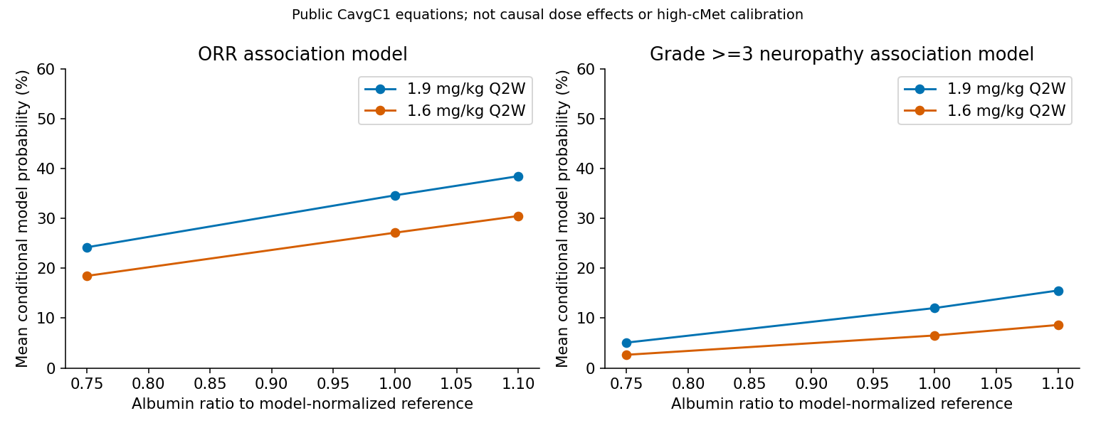
Figure 2. ORR and PN model projections across albumin ratios, calculated by the author.
This figure does not establish that low albumin means lower clinical risk. Only the specified PK pathway changes. Pathways involving nutritional status, disease burden and comorbidities are absent.
The dose ranking depends on value judgments
Putting the two models side by side does not choose between 1.9 and 1.6 mg/kg. For illustration, I used an additive score:
\[ U=p_{ORR}-\lambda p_{PN\ge3} \]
The weight \(\lambda\) expresses a hypothetical penalty for PN, rather than a patient-derived utility. Because the ORR and PN equations come from different analysis populations, this score is not a net clinical benefit in one population. It also does not calculate the probability of response without PN.
With nominal coefficients at albumin ratio one, the mean scores were equal at:
\[ \lambda^*=\frac{0.07493}{0.05501}=1.36 \]
The corresponding weights were 2.35 at ratio 0.75 and 1.16 at ratio 1.10. These are not discoveries of an optimal dose. They quantify how the ranking changes with the valuation built into the calculation.
Marginal confidence intervals do not reconstruct joint uncertainty
Marginal 95% confidence intervals for the exposure–response coefficients are public, but I could not verify intercept–slope covariance. Independently sampling those intervals would not produce a justified 95% prediction interval.
Instead, I placed nine points within each coefficient's marginal interval, producing 81 coefficient combinations per model. Combining the resulting ORR and PN score differences showed that the nominal ranking was unstable across this sensitivity grid.
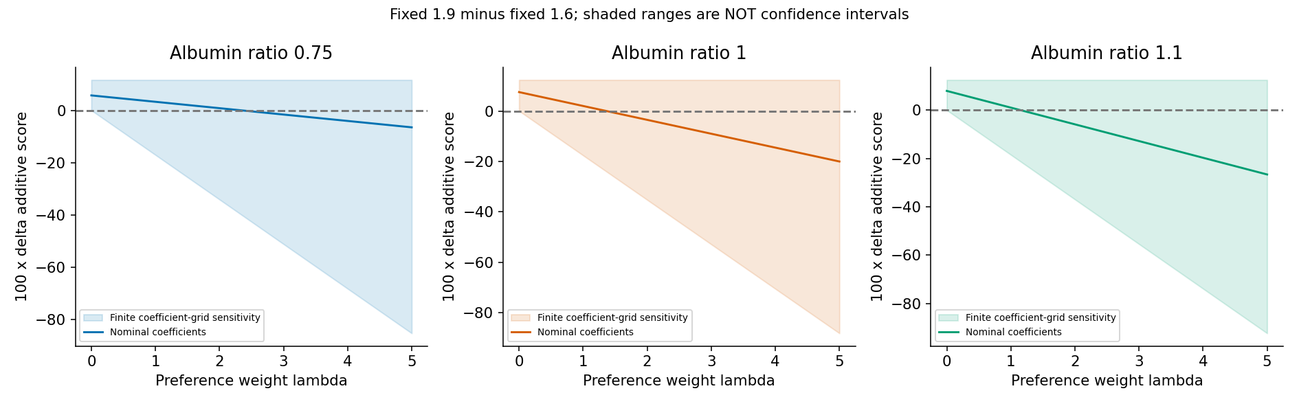
Figure 3. Sensitivity to toxicity weights and a finite coefficient grid; the band is not a confidence interval.
The band spans finitely many coefficient scenarios. It is neither a joint 95% interval nor a guaranteed bound over the entire continuous parameter region. It may include implausible combinations of strongly correlated coefficients, and no probability weights were assigned. It cannot yield the probability that either dose should be selected. That requires information such as coefficient covariance and patient-level exposure and outcomes.
ADC and MMAE can move in opposite directions
The published albumin coefficients on clearance differ: −0.970 for ADC and 1.99 for unconjugated MMAE. Holding dose and formation scale constant gives the following relative steady-state AUC values at albumin ratio 0.75.
Table 5. Algebraic relative exposure at albumin ratio 0.75.
| Component and condition | Steady-state AUC relative to reference |
|---|---|
| ADC | 0.757 |
| MMAE, reference renal function | 1.773 |
| MMAE, moderate/severe renal impairment coefficient applied | 2.348 |
These are algebraic ratios from the clearance covariate equations. I could not sufficiently establish the absolute MMAE formation scale or its interindividual dependence with ADC, so I did not reproduce absolute MMAE concentrations or a complete linked model. Disease-dependent changes in formation would also invalidate the comparison's assumption.
The PN equation here uses ADC exposure. I did not translate the MMAE ratios into PN risk. The FDA separately examines tumor burden, opposite ADC/MMAE exposure relationships and exploratory fatal-adverse-event findings. ORR and PN cannot represent the entire safety profile (3, pp. 227–235).
Initial lower dosing remains unresolved by this equation
Fixed 1.6 and the first-two-dose reduction have identical histories during the first 14 days. They therefore have the same \(C_{\mathrm{avg,C1}}\) and the same outputs from these ORR and PN equations.
Their later exposures differ. Equal model outputs are not evidence of equal long-term outcomes. The input contains no information that distinguishes later dosing history, and substituting later exposure into an initial-exposure equation does not repair that limitation.
The public models support separating early exposure reduction from later recovery. They show that fixed-dose comparisons depend on value judgments and coefficient uncertainty. They do not support repurposing this static exposure–response equation to predict the outcomes of sequential dose escalation. Establishing the efficacy and safety of a new regimen lies beyond this calculation.
Data and code availability
The Python analysis checked an independent ODE solution, finite-infusion integration, mass balance, dose proportionality and identical first-cycle exposure. The package distributes numerical inputs, original code and generated figures and tables, without redistributing original-paper figures or patient records.
Analysis code, inputs, summary tables and rerun instructions
References
- US Food and Drug Administration. FDA grants accelerated approval to telisotuzumab vedotin-tllv for NSCLC with high c-Met protein overexpression. 2025 May 14. Approval information.
- Babel H, Brunsdon P, Engelhardt B, Schmitt V, Ratajczak C, Mensing S, et al. Population Pharmacokinetics and Exposure‐Response Analyses for Telisotuzumab Vedotin in Patients With c‐Met Protein Overexpressing Tumors. CPT: Pharmacometrics & Systems Pharmacology. 2026;15(3):e70219. doi:10.1002/psp4.70219.
- US Food and Drug Administration. Telisotuzumab vedotin-tllv: multidisciplinary review, application 761384. 2025. Tables 47, 48, 51 and 54; pp. 227–235. Review report.