Repotrectinib escalation timing: exploring lead-in regimens with a public population PK model
An independent Python implementation of published structural equations compares 7-, 14- and 21-day lead-ins. Conditional paired simulations and sensitivity analyses separate cumulative exposure, peak-window effects and late troughs. No patient refitting, NONMEM equivalence or efficacy/safety prediction is claimed.
On this page
- Question and scope of use
- Public information used
- Calculating autoinduction
- Three dosing histories
- Cumulative exposure and later troughs give different answers
- Compare within the same virtual patient
- Which comparisons depend on assumptions?
- Later troughs lose distinctions in the lead-in history
- Numerical checks and remaining limitations
- References
Literature checked on October 11, 2026. These simulations use published estimated parameters, rather than refitting patient-level data. Reported findings, my calculations and their interpretation are distinguished below.
Repotrectinib is a ROS1/TRK inhibitor used for ROS1 fusion-positive non-small-cell lung cancer and NTRK fusion-positive solid tumors. Treatment starts at 160 mg once daily for 14 days before increasing to twice daily. Clearance increases after treatment begins through CYP3A autoinduction (1, 2). The empirical PopPK model used here represents that change as a function of time and concentration, rather than directly modeling CYP3A enzyme synthesis and degradation. The path to the final dose therefore matters as well as the final dose itself.
Where would differences appear if the lead-in lasted seven or 21 days?
Under the conditions examined here, cumulative exposure over 28 days differed, while trough concentrations at the end of day 28 were almost identical. This does not establish a benefit of earlier escalation or the safety of later escalation. It shows how exposure metrics reveal different aspects of a regimen and helps identify observations needed for comparison.
Question and scope of use
| Item | Definition |
|---|---|
| Quantity of interest | How do 28-day AUC, intervening peaks and end-of-period trough change when 160 mg once daily continues for seven, 14 or 21 days before twice-daily dosing? How much does the comparison depend on interindividual variability, fixed effects and food assumptions? |
| Context of use | Exploratory exposure comparison with a public model, to clarify exposure metrics and sampling periods for research on lead-in regimens. These results alone do not select clinical doses, predict individual adverse events or determine whether to conduct a comparative trial. |
The question is when and with what measurements candidate regimens need to be distinguished. Without comparative efficacy and safety data, exposure differences do not establish which regimen is preferable.
Public information used
| Material | Use here | Not used |
|---|---|---|
| Du et al. 2025 PopPK paper (1), Table 2 | Final estimates and reported interindividual variability | Original individual concentrations or patient-specific estimates |
| Data S3 of that paper | Cross-check absorption lag, concentration units, autoinduction and patient/healthy-volunteer distinction | NONMEM refitting |
| Du et al. 2025 exposure–response analysis (3) | Check original exposure metrics and how extrapolation here differs | Extrapolated ORR, PFS or adverse-event probabilities for other regimens |
| 2026 TRIDENT-1 safety analysis (4) | Check adverse events and failure to escalate during the lead-in | Reconstruction of individual events from aggregate data |
Supplements were obtained through Europe PMC's public distribution. Original text and figures are not reproduced; the figures and calculation code below were created independently. Without patient-level data, this is neither new model estimation nor external validation against patient concentrations.
Calculating autoinduction
The reference individual is an adult patient weighing 70 kg receiving oral doses. Food is initially fixed to fasted; other categories are compared later. The model has first-order absorption with lag and two distribution compartments:
\[ \frac{dA_g}{dt}=-k_aA_g \] \[ \frac{dA_c}{dt}=k_aA_g-\frac{CL(t)}{V_c}A_c-Q\left(\frac{A_c}{V_c}-\frac{A_p}{V_p}\right),\qquad \frac{dA_p}{dt}=Q\left(\frac{A_c}{V_c}-\frac{A_p}{V_p}\right) \]
Fraction F of each dose enters the absorption compartment after the lag. Amounts are in mg and concentrations in ng/mL, so \(C(t)=1000A_c/V_c\).
With predose concentration \(C_{\rm pre}\), autoinduction is calculated as (1)
\[ CL(t)=CL_0\exp\left\{ I_{\max}\frac{C_{\rm pre}}{EC_{50}+C_{\rm pre}} \frac{t}{TC_{50}+t} \right\} \]
\(C_{\rm pre}\) is updated at each dose event and held until the next dose. Time \(t\) runs from the first dose and does not reset at escalation. Here \(EC_{50}\) is an autoinduction-model constant, not an antitumor efficacy threshold.
| Parameter | Value | Unit and meaning |
|---|---|---|
| \(CL_0\) | 7.1 | L/h, before autoinduction |
| \(V_c\), \(V_p\) | 19.8, 221 | L, patient central and peripheral volumes |
| \(Q\) | 4.98 | L/h, intercompartmental clearance |
| \(k_a\), F | 0.0541, 0.52 | 1/h and dimensionless; fasted |
| Absorption lag | 0.421 | h |
| \(I_{\max}\) | 1.59 | Dimensionless term inside the CL exponent |
| \(EC_{50}\), \(TC_{50}\) | 77, 47.2 | ng/mL and h |
Values are the final estimates in original Table 2, rather than initial estimates in the supplementary control stream. \(I_{\max}=1.59\) does not mean a maximum 1.59-fold clearance increase: at sufficiently high concentration and time, the multiplier approaches \(\exp(1.59)\).
I ported the equations into Python and retained predose concentrations at exact event times. The original NONMEM $PK block is evaluated per record; its stated order calculates CL before updating the retained concentration at dosing. Without the original observation records or NONMEM execution, I do not claim complete reproduction of the original program. The main analysis uses the latest predose concentration and continuously updates the time term. Sensitivity analyses hold CL between dosing events, or use dose records alone with the order “calculate CL using the previous retained concentration, then retain the current concentration.” The latter also does not reproduce an original run containing observation records.
Three dosing histories
The first dose is at time zero. Twice-daily dosing begins at 168, 336 or 504 h after seven-, 14- or 21-day lead-ins, respectively: Days 8, 15 and 22. The 28-day window is 0–672 h; its final trough is immediately before the Day 29 dose.
| Lead-in | Total dose over 28 days (mg) | AUC0–28 days (ng·h/mL) | Predose Day 29 (ng/mL) |
|---|---|---|---|
| 7 days | 7,840 | 201,065 | 251.1 |
| 14 days | 6,720 | 178,977 | 251.0 |
| 21 days | 5,600 | 158,500 | 250.0 |
Earlier escalation also increases total 28-day dose. Relative to the 14-day lead-in, total dose is 16.7% higher after seven days and 16.7% lower after 21 days. This comparison changes both lead-in length and its resulting total dose; it does not isolate dosing interval at an equal total dose.
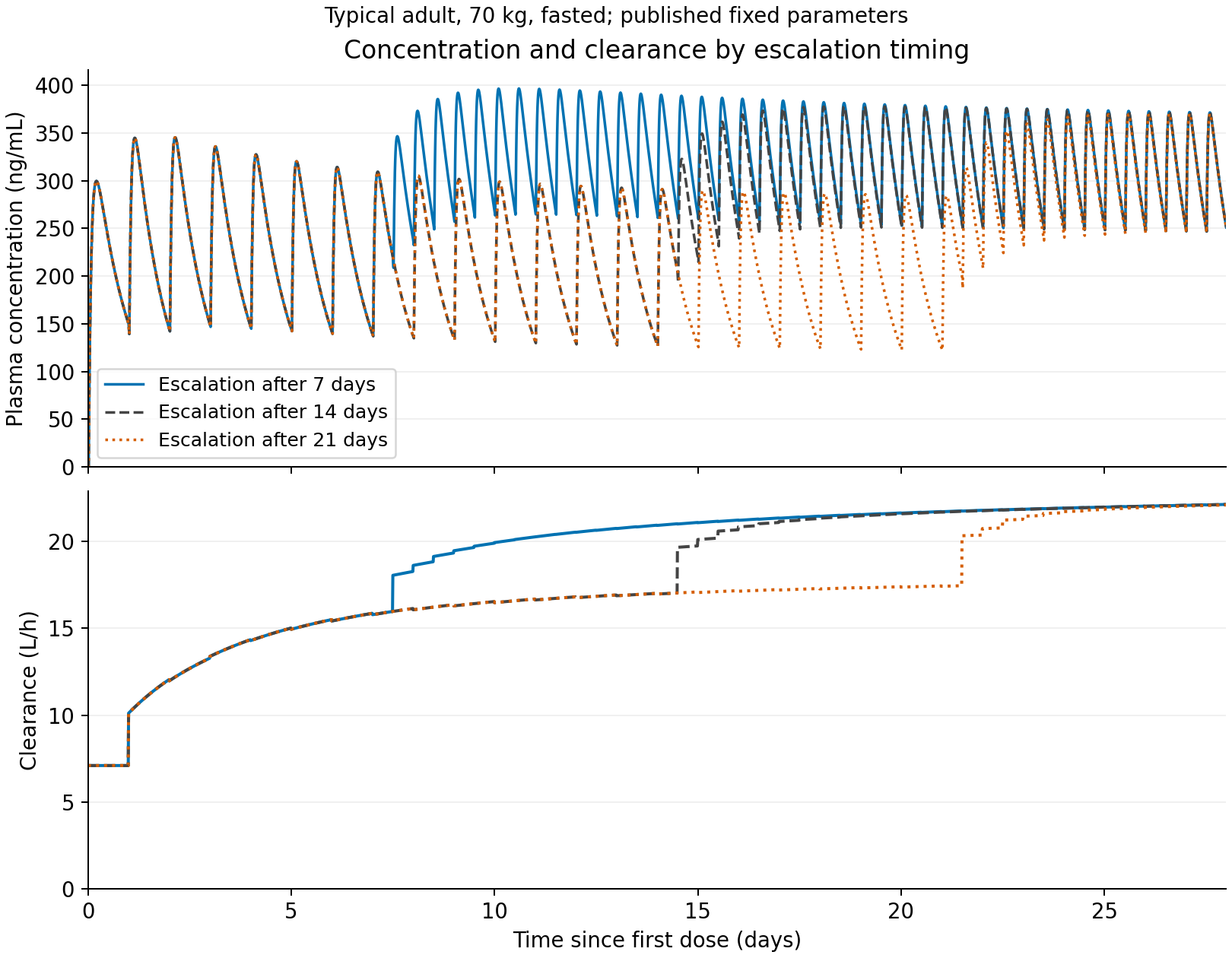
Figure 1. Typical fixed-effect predictions for a fasted 70-kg adult. Blue, gray and orange indicate seven-, 14- and 21-day lead-ins. No patient observations or confidence intervals are shown. Outputs: analysis/run_analysis.py, outputs/tables/typical.csv.
Cumulative exposure and later troughs give different answers
The seven-day lead-in gave 1.123 times the 28-day AUC of the 14-day lead-in; the 21-day lead-in gave 0.886 times. Day 29 predose concentration ratios were 1.0002 and 0.9959, respectively. Later twice-daily dosing narrows concentration differences, while AUC retains exposure accumulated earlier.
Similar later troughs do not mean equal exposure during the lead-in. A single late measurement can miss differences along the way.
The peak in the first seven days was identical across schedules. Dosing histories were identical until then: this is an implementation check, rather than a new finding.
Comparing only peaks on Days 8–21 excludes post-escalation observations for the 21-day lead-in. That window alone cannot establish that later escalation suppresses peaks. I separately calculated peaks during the 72 h after each escalation.
| Lead-in | Days 8–21 peak (ng/mL) | Peak within 72 h after each escalation (ng/mL) | Maximum over days 0–28 (ng/mL) |
|---|---|---|---|
| 7 days | 396.7 | 395.3 | 396.7 |
| 14 days | 377.9 | 373.4 | 377.9 |
| 21 days | 309.3 | 364.1 | 370.3 |
Event-aligned windows fall on different calendar days, at different stages of autoinduction and accumulation. This is therefore not a dose comparison from the same state either. Calendar-aligned and escalation-aligned metrics both need to be shown.
Compare within the same virtual patient
I generated a conditional population of 256 virtual individuals using published variability in CL, central volume, intercompartmental CL, absorption rate and F. Weight and food were fixed; each individual's random effects were shared across schedules. Peripheral-volume random effects were set to zero following the supplement.
| Lead-in | Metric | Median ratio | 5th–95th percentiles |
|---|---|---|---|
| 7 days | 28-day AUC | 1.125 | 1.110–1.147 |
| 7 days | Days 8–21 peak; pre-escalation only for the 21-day lead-in | 1.049 | 1.035–1.058 |
| 7 days | Predose Day 29 | 1.000 | 1.000–1.003 |
| 7 days | Peak within 72 h after each escalation | 1.057 | 1.043–1.073 |
| 21 days | 28-day AUC | 0.884 | 0.865–0.897 |
| 21 days | Days 8–21 peak; pre-escalation only for the 21-day lead-in | 0.799 | 0.712–0.905 |
| 21 days | Predose Day 29 | 0.996 | 0.984–1.000 |
| 21 days | Peak within 72 h after each escalation | 0.975 | 0.969–0.982 |
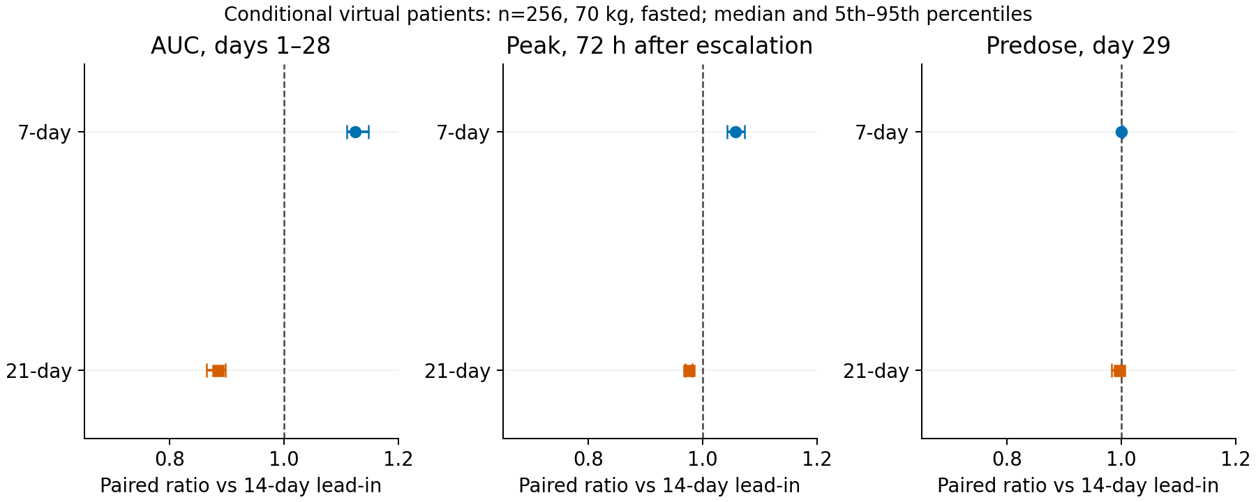
Figure 2. Ratios against the 14-day lead-in within each virtual patient. The middle panel uses the 72-hour post-escalation peak, avoiding a window that includes only pre-escalation observations. Points are medians and lines 5th–95th percentiles. All panels share the horizontal range. These are neither 95% confidence intervals for parameter estimates nor predictive intervals for an actual patient population. Output: outputs/tables/paired.csv.
The direction of the 28-day AUC differences persisted in this conditional population. This depends on fixed food and weight and independent random effects. It does not reconstruct real covariate distributions, changing food conditions, interruptions or reductions. Residual error was not added.
Which comparisons depend on assumptions?
I moved fixed effects one at a time to the lower and upper limits of their published 95% intervals in Table 2. Without estimation covariance, I did not sample these independently and call the result an estimation-uncertainty distribution.
| Lead-in | Metric | Minimum–maximum ratio against 14 days |
|---|---|---|
| 7 days | 28-day AUC | 1.119–1.128 |
| 7 days | Days 8–21 peak; pre-escalation only for 21 days | 1.027–1.069 |
| 7 days | Predose Day 29 | 1.000–1.000 |
| 21 days | 28-day AUC | 0.881–0.890 |
| 21 days | Days 8–21 peak; pre-escalation only for 21 days | 0.800–0.836 |
| 21 days | Predose Day 29 | 0.995–0.997 |
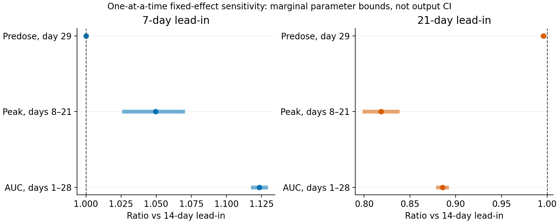
Figure 3. Points use reference parameters; lines give minima and maxima across 20 one-at-a-time changes. Joint parameter changes are not included, and these are not output confidence intervals. Output: outputs/tables/sensitivity.csv.
Food categories required more caution. Using their published F and absorption rates retained the direction of AUC differences, but changed the Days 8–21 peak comparisons.
| Model food category | 7-day AUC ratio | 21-day AUC ratio | 7-day Days 8–21 peak ratio | 21-day Days 8–21 peak ratio |
|---|---|---|---|---|
| fasted | 1.123 | 0.886 | 1.050 | 0.818 |
| fed | 1.109 | 0.901 | 1.058 | 0.995 |
| modified | 1.105 | 0.904 | 1.032 | 1.000 |
| unknown | 1.102 | 0.906 | 1.000 | 1.000 |
“Unknown” represents observations with unknown food status, not a deliberately selectable meal condition. Category differences should not be read as intervention effects of changing an individual's food intake.
Holding CL between dose events produced AUC ratios of 1.123 and 0.886 for seven and 21 days. Using dose records alone with the supplement's CL/concentration update order gave 1.122 and 0.887. Both were close to the main analysis here. Removing autoinduction as a diagnostic control gave 1.183 and 0.821. The latter is a computational control for the contribution of the autoinduction term, rather than another fitted model. Output: outputs/tables/scenarios.csv.
These results establish the direction of AUC differences only under the examined conditions. They do not establish robustness to unmeasured PD or alternative mechanistic autoinduction models.
Later troughs lose distinctions in the lead-in history
| Candidate sampling time for the typical patient | 7 days (ng/mL) | 14 days (ng/mL) | 21 days (ng/mL) |
|---|---|---|---|
| Predose Day 15 | 265.8 | 128.5 | 128.5 |
| Predose Day 22 | 256.4 | 255.3 | 124.3 |
| Predose Day 29 | 251.1 | 251.0 | 250.0 |
The candidate differences look different before doses on Days 15 and 22 than on Day 29. These are illustrative sampling times showing which portions of the history can be lost, rather than an optimized sampling design.
The table gives predose concentrations, not absorption-phase peaks. Sampling counts and times, or required sample sizes, were not optimized. Errors in dosing, food and interruption histories were not included.
Safety timing also matters. In the 2026 TRIDENT-1 analysis, median time to dizziness onset was seven days, and 66 of 472 patients did not escalate from once- to twice-daily dosing (4). This does not prove earlier escalation harmful, but it demonstrates why events during the lead-in cannot be represented solely by post-escalation steady-state exposure.
The published E–R analysis uses mean exposure over the first 56 days for ORR and time-dependent cumulative mean exposure for PFS and safety (3). The present 28-day AUC and peak cannot be substituted directly into those prediction equations. I calculated neither response nor adverse-event probabilities.
Numerical checks and remaining limitations
Calculations used Python, NumPy, SciPy and Matplotlib. Checks covered dose amounts, nonnegative drug amounts and mass balance across absorption, central, peripheral and eliminated amounts. With autoinduction removed, results were compared with an independently constructed linear-model matrix-exponential solution. The main analysis used fourth-order Runge–Kutta, with SciPy's adaptive solver as a separate check.
Six numerical tests passed. Between solvers, the largest relative difference in reference AUC or final trough was 2.1e-08%; maximum mass-balance error was 4.1e-12 mg. Halving the step also made little difference to either metric. Steps were capped for the whole virtual population to avoid instability with small volumes. Output: outputs/verification.json.
These validate numerical implementation, not patient concentrations or clinical events. Original population averages, EBE-derived exposure and prescribing-information reference values have different weight, food and patient conditions. I did not force a typical-patient calculation to match them and call that successful reproduction.
Remaining limitations include absent individual observations and dosing histories, absent estimation covariance, no rerun of the original NONMEM code and no clinical validation of alternative escalation times. Seven- and 21-day lead-ins are hypothetical research conditions, not recommended regimens.
Reading lead-in differences from later troughs alone misses early cumulative exposure. Whether more early exposure is worthwhile requires a separate question about efficacy and safety over time. This analysis stops at distinguishing the metrics and observation periods needed for that comparison.
References
- Du S, et al. A Novel Empirical Autoinduction Model to Characterize the Population Pharmacokinetics and Recommend Dose for Repotrectinib in Adult and Adolescents With Advanced Solid Tumors Harboring ALK, ROS1, or NTRK1–3 Rearrangements. CPT: Pharmacometrics & Systems Pharmacology. 2025;14:1179–1190. doi:10.1002/psp4.70036. Open full text and supplements.
- FDA Drug Trials Snapshot: AUGTYRO.
- Du S, et al. Exposure–Response Analysis of Repotrectinib to Support the Dose Recommendation for Patients With ROS1-Positive NSCLC or NTRK-Positive Solid Tumors. CPT: Pharmacometrics & Systems Pharmacology. 2025;14:1993–2005. doi:10.1002/psp4.70102. Open full text.
- Characterization and clinical management of adverse events following treatment with repotrectinib: a TRIDENT-1 analysis. The Oncologist. 2026;31:oyag137. doi:10.1093/oncolo/oyag137. Open full text.
Calculation code, numerical tables and reproduction instructions
Cite this article
Kumakura, D. (2026). Repotrectinib escalation timing: exploring lead-in regimens with a public population PK model. daikikumakura.github.io. https://daikikumakura.github.io/writing/repotrectinib-escalation-en.html