RAS inhibitor dosing: from public PK/PD data to target-coverage scenarios
On this page
- Abstract
- Introduction
- Methods and results
- Scope and sources
- Reconstructing the mouse blood–tumor–pathway model
- Virtual-drug assumptions
- Population coverage metrics and results
- Where dose splitting changes the answer
- Exposure cost and administration burden
- Sensitivity to unmeasured properties
- Sensitivity to nonlinear and time-dependent PK
- An exposure–outcome association is not automatically causal
- Numerical checks
- Discussion
- Conclusion
- Data and code availability
- References
Abstract
I reconstructed a public mouse blood–tumor–DUSP6 model, then compared explicitly hypothetical QD, BID and TID regimens. The analysis separates three questions: whether the published implementation can be reproduced, what follows mathematically from assumed PK/PD, and what remains unqualified for a new molecule.
The main finding is conditional: plasma half-life alone does not determine dosing frequency. Distribution, potency, target turnover and the lower tail of exposure matter. In a reference virtual population, dividing the same daily amount increased the proportion maintaining a concentration threshold for at least 90% of the interval from 20.6% to 61.5%. Those are simulation results, not clinical response rates or a recommendation for daraxonrasib.
Introduction
At the same total daily dose, how much can dividing an oral dose change sustained target inhibition? And what would need to be measured before applying that comparison to a new RAS inhibitor?
Question and intended use
Question of interest: at matched normalized daily amount, when does dose splitting materially change population target coverage, and which unmeasured properties could change that conclusion?
Context of use: public-evidence reconstruction and research/learning scenarios for model development. This analysis does not select a first-in-human starting dose, establish a therapeutic window, or predict patient efficacy or toxicity. “Material” below means an illustrative 10 percentage-point difference in coverage; it is not a clinical minimum important difference.
The central comparison is between virtual molecules, rather than a pooled model of different RAS drugs. A reversible RAS(ON) inhibitor and a covalent KRAS inhibitor cannot be treated as interchangeable observations simply because both act on RAS signaling.
Methods and results
Scope and sources
Table 1. Evidence and boundaries
| Evidence | Usable information | Boundary |
|---|---|---|
| Daraxonrasib/RMC-6236 mouse supplement | Blood, tumor and DUSP6 group means; equations; point estimates | Sparse means are not repeated individual observations |
| Daraxonrasib human label | Summary systemic PK at a stated clinical dose | Not an individual-data PopPK dataset or tumor PK model |
| RMC-7977 study | Mechanistic context and downloadable source data | Not a human population distribution for another molecule |
| Olomorasib clinical study | Compound-specific exposure and dosing observations | Cannot identify turnover parameters for a new inhibitor |
| Virtual analysis here | Transparent paired comparisons under stated assumptions | Does not estimate drug-specific clinical parameters |
The RMC-6236 paper describes fitting sparse mean profiles, formed from three animals per time point. This matters: the dataset can support structural reconstruction, but it cannot recover a human random-effects distribution. I downloaded the publisher-hosted Supplementary Methods and Tables S8/S9; Table S9 yielded 72 dosing/observation records across model-development and separate validation groups. The original study (1) explains the experimental and modeling context.
I also checked the published correction (2). It addresses a figure-label problem and cell-panel methods. The downloaded 2024 and 2025 versions of the five selected supplements had identical file hashes. That comparison checks file identity; it does not resolve every ambiguity in the equations.
RMC-7977 source data were available through the Nature study (3). I retained them in the source audit, but did not use them to manufacture longitudinal human PK. The olomorasib study (4) reports an approximately three-hour half-life and a BID program, including modeled TEC80 coverage. This is compound-specific evidence, not proof that every short-lived inhibitor requires BID or that covalent binding automatically permits QD.
Reconstructing the mouse blood–tumor–pathway model
The model combines oral one-compartment blood PK with tumor exchange and an indirect DUSP6 response. With amounts in the absorption and blood compartments, \(A_a,A_b\), blood concentration \(C_b=A_b/V\), tumor concentration \(C_t\), and DUSP6 percentage \(E\):
\[ \frac{dA_a}{dt}=-k_aA_a,\qquad \frac{dA_b}{dt}=k_aA_a-CL\,C_b \]
\[ \frac{dC_t}{dt}=k_{pt}f_u\frac{C_b}{BP(C_b)}-k_{tb}C_t \]
\[ \frac{dE}{dt}=100k_{out}\left(1-\frac{C_t}{IC_{50}+C_t}\right)-k_{out}E. \]
Table 2. Published mouse-model parameters
| Quantity | Value used | Role |
|---|---|---|
| \(k_a\) | 0.648316 h⁻¹ | Absorption |
| \(V/F\) | 10.199248, printed as L | Apparent volume; normalization caveat below |
| \(CL/F\) | 2.910761 L/h | Apparent blood clearance |
| \(k_{pt}\), \(k_{tb}\) | 115, 0.1 h⁻¹ | Tumor exchange |
| \(f_u\) | 0.011 | Mouse unbound plasma fraction |
| \(IC_{50}\) | 42.261016 nM | Tumor concentration–DUSP6 inhibition |
| \(k_{out}\) | 2.385655 h⁻¹ | DUSP6 turnover |
These point estimates come from Supplementary Table S8; equations and binding assumptions come from the Supplementary Methods. Parameter-estimate CVs describe estimation precision; I did not reinterpret them as individual variability.
Two source ambiguities deserve attention. First, S9 doses are nmol/kg while S8 labels apparent volume as L. The calculation uses the printed numbers with the implicit dose normalization needed to obtain nM; a complete unit-consistent implementation specification would strengthen this reconstruction. Second, Methods implement
\[ BP(C_b)=5.5-\frac{5.2C_b}{1819+C_b}, \]
whereas the mouse binding table prints an IC50 of approximately 1.8188 with an nM label. Those denominators differ by roughly 1,000-fold. I used the printed Methods expression as the primary implementation and the literal table value as a sensitivity scenario, without silently correcting either source. Tumor concentration here is total concentration; the source's exchange terms do not establish an identifiable unbound tumor partition coefficient.
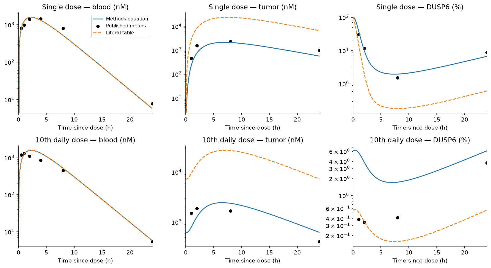
Figure 1. Original reconstruction using Supplementary Table S9 group means. The alternative denominator affects tumor/PD calculations, not blood PK. Points are group means, not longitudinal individual profiles. The logarithmic axis makes relative discrepancies visible.
Figure 1 and Table 3 compare the reconstruction with source means. Across positive observations in all extracted PK/PD groups, the median absolute relative errors were:
Table 3. Descriptive reconstruction residuals
| Endpoint | Observations | Methods denominator | Literal table denominator |
|---|---|---|---|
| Blood concentration | 43 | 25.9% | 25.9% |
| Tumor concentration | 30 | 45.2% | 557.4% |
| DUSP6 expression | 30 | 62.8% | 80.5% |
These are descriptive reconstruction residuals, not goodness-of-fit estimates from a new likelihood. The same parameters were used for development and validation groups; no parameter was retuned to make the plots agree. Near-zero DUSP6 values amplify relative error, so the table should be read with the original-scale curves and downloadable residuals. A file that runs is not automatically a qualified predictive model. This reconstruction is incomplete, especially for tumor/pathway prediction.
A separate human summary check
The FDA label (5) reports, at 300 mg QD, AUC 3,760 ng·h/mL, Cmax 365 ng/mL, median Tmax 2.2 h, terminal half-life 9.2 h, and apparent clearance 80.4 L/h. These systemic summaries should not be mixed with mouse whole-blood observations.
As a deliberately limited check, I combined clearance and terminal half-life into a one-compartment approximation and solved absorption rate to match single-dose Tmax. Its periodic QD AUC was 3,731 ng·h/mL, but peak concentration was 287.8 ng/mL, about 21% below the label summary. Agreement in AUC follows largely from dose/clearance; it does not validate the concentration–time shape. Terminal half-life, mean clearance and median Tmax also need not describe one shared typical patient. I therefore did not transfer this approximation into a claimed human tumor-response model.
Virtual-drug assumptions
The following models are assumptions used to understand design dependencies. They are not an estimated PopPK prior for RAS inhibitors.
Table 4. Virtual-drug assumptions
| Assumption | Reference | Sensitivity |
|---|---|---|
| Apparent normalized volume | 1 | No independent volume variability modeled |
| Absorption rate | 1 h⁻¹ | 0.5–2 h⁻¹ |
| Plasma half-life | 4 h | 2–24 h |
| Reference mean concentration / C90 | 3 | 0.25–8 phase grid |
| Clearance CV | 40% | 20%, 60% |
| Relative exposure multiplier CV | 30% | Multiplicative exposure shifts |
| Tumor/plasma ratio | 1 | 0.5, 2; wider global range |
| Tumor equilibration half-life | Instantaneous | 2, 8 h |
| Target turnover half-life | 24 h | 6, 72 h |
Clearance and the relative exposure multiplier have independent lognormal distributions with median 1. The latter can exceed 1; it is not absolute oral bioavailability. The nominal ratio of 3 refers to the reference subject, not the arithmetic mean of the simulated population. There is no residual observation error because the task is a latent-exposure comparison, not fitting observations.
For elimination rate \(k=\log(2)/t_{1/2}\), interval \(\tau\), and normalized per-dose amount \(D\), periodic oral concentration is
\[ C_{ss}(t)=\frac{Dk_a}{V(k_a-k)} \left[\frac{e^{-kt}}{1-e^{-k\tau}}- \frac{e^{-k_at}}{1-e^{-k_a\tau}}\right],\quad 0\le t\le\tau. \]
At a fixed point in the scenario space, QD, BID and TID have identical total daily amount. Linear systemic AUC is therefore unchanged within each paired subject. On the phase diagram, half-life and reference exposure ratio vary together as coordinates; daily amount is adjusted between grid points to maintain the requested reference ratio. The separate global sensitivity experiment instead holds daily amount fixed when half-life changes.
Three different meanings of persistent inhibition
For reversible concentration-driven inhibition,
\[ I(t)=\frac{C_t(t)}{1/9+C_t(t)}. \]
The assumed C90 is normalized to 1. For a delayed pathway response, normalized remaining activity \(R\) follows \(dR/dt=k_{out}[1-I(t)-R]\). For covalent target inhibition, remaining uninhibited target \(U\) follows
\[ \frac{dU}{dt}=k_{deg}(1-U)- \frac{k_{inact}C_t(t)}{K_I+C_t(t)}U,\qquad TE=1-U. \]
The covalent reference assumes \(K_I=1\) and \(k_{inact}=18\log(2)/24\) h⁻¹, so constant concentration 1 gives 90% inhibition at a target-turnover half-life of 24 h. This matches one steady-state reference point, not the entire concentration–response curve. The nonlinear models differ in more than memory, so differences cannot be attributed solely to “reversible versus covalent.” This covalent equation is never assigned to daraxonrasib.
Tumor equilibration sensitivity uses \(dC_t/dt=k_t(K_pC-C_t)\). It explores filtering and retention, without claiming that a selected \(K_p\) has been measured in human tumors.
Population coverage metrics and results
For each virtual subject, TAT is the fraction of a dosing interval above the assumed effect threshold. Reversible inhibition uses concentration ≥ C90; persistent models use inhibition ≥ 90% directly. PTC90 is the fraction of subjects whose TAT is at least 90%. Thus the two “90” criteria have different roles. PTC80/PTC95 vary the required fraction of time while retaining the same effect threshold.
I also report trough concentration, peak concentration, systemic AUC and a normalized below-threshold deficit. A deficit of zero means no threshold shortfall; it is not zero clinical risk. Coverage probabilities are conditional on the assumed distributions and thresholds.
Primary scenarios use 10,000 virtual subjects and the same random draws for each regimen. Paired differences use the standard error of within-subject attainment differences, rather than treating QD and BID as independent populations.
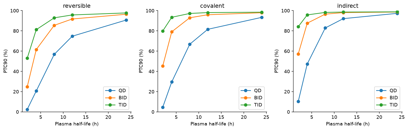
Figure 2. PTC90 under three explicitly hypothetical mechanisms; reference exposure ratio 3, clearance CV 40%, relative exposure CV 30%. Target/pathway turnover half-life is 24 h where applicable.
Table 5. Sustained population coverage
| Half-life | Model | QD PTC90 | BID PTC90 | BID − QD |
|---|---|---|---|---|
| 4 h | Reversible | 20.6% | 61.5% | +40.9 pp |
| 4 h | Covalent | 29.6% | 79.1% | +49.5 pp |
| 4 h | Delayed pathway | 47.3% | 87.6% | +40.3 pp |
| 8 h | Reversible | 56.8% | 85.5% | +28.7 pp |
| 24 h | Reversible | 90.7% | 96.4% | +5.7 pp |
Figure 2 and Table 5 compare the hypothetical mechanisms. For the four-hour reversible reference, the paired Monte Carlo SE of the BID−QD difference is approximately 0.49 percentage points. Monte Carlo uncertainty is small relative to this difference, but model uncertainty is not represented by that SE. Average normalized daily AUC is approximately 80.4 under both schedules; average peak falls from 9.28 to 5.50. This isolates a concentration-profile change under linear PK rather than an increase in total exposure.
Persistence does not produce a universal answer. With the covalent model's inactivation rate held fixed, changing target turnover from 24 to 72 h raises QD PTC90 from 29.6% to 93.4%; BID then reaches 100% in this finite virtual sample. At a six-hour turnover half-life, neither schedule reaches PTC90: with the assumed fixed inactivation rate, the saturation ceiling is only 81.8% inhibition, so increasing concentration cannot reach the 90% threshold. Fast target replacement can defeat sustained inhibition; slow replacement can reduce the gain from splitting. A 100% simulation result is not proof of universal coverage.
Where dose splitting changes the answer
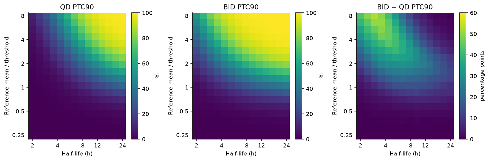
Figure 3. Reversible model, 14 half-life values × 18 reference exposure ratios, 2,000 subjects per grid point. Colors are probabilities or percentage-point differences; these are exploratory grid coordinates, not clinical dose boundaries.
In Figure 3, the largest gains occur where troughs are limiting but greater exposure can plausibly cross the threshold. If nearly everyone is below threshold even with BID, splitting cannot compensate for insufficient average exposure. If QD already covers almost everyone, the incremental coverage gain is small. This explains why “short half-life means BID” is an incomplete rule.
A 10 pp convention classifies 48.0% of the sampled grid as having a material gain. Using 5 or 20 pp changes that to 60.7% or 30.2%. These are grid fractions, not proportions of possible drugs or patients: they depend on the chosen ranges and spacing.
The maximum pointwise binomial Monte Carlo SE on a 2,000-subject grid is about 1.12 pp. At three selected reference/boundary points, 10,000-subject, finer-integration checks changed individual PTC90 estimates by up to 2.79 pp. The coarse diagram is suitable for broad patterns, not a sharply estimated decision contour. All probabilities and checks are included in the accompanying tables.
Exposure cost and administration burden
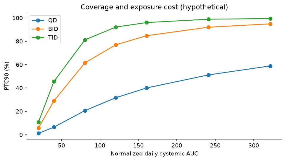
Figure 4. Twenty-one assumed actions. Lines connect amounts within a schedule; they are not treatment recommendations.
The mathematical Pareto comparison in Figure 4 uses four objectives: greater PTC90, lower daily AUC, lower peak, and fewer administrations. Splitting may improve coverage and reduce peak while requiring more administrations. Increasing total daily amount raises exposure burden. Without a measured safety relationship and preferences over these consequences, there is no justified single “optimal” action. Peak and AUC here are exposure costs, not predicted adverse events.
The downloadable table marks non-dominated actions. Calling an action non-dominated means another sampled action does not improve every specified objective. It does not establish clinical superiority, and a larger action set could change the frontier.
Sensitivity to unmeasured properties
The local sensitivity table varies clearance CV, tumor partition and equilibration, and target turnover. A separate Latin-hypercube design samples 400 parameter sets, using 512 paired subjects per set and a fixed daily amount. It varies half-life, clearance and exposure multipliers, tumor partition, potency, absorption and target turnover over stated ranges.
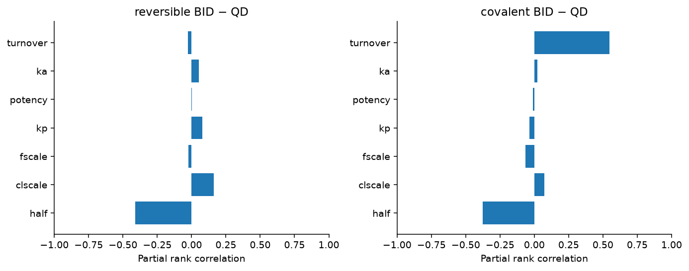
Figure 5. PRCC screening depends on the sampled ranges and model. A coefficient close to zero can conceal a nonmonotonic dependence.
For Figure 5, I used partial rank correlation as a screening tool, following the methodology discussed by Marino and colleagues (6). It is most informative for monotonic relationships. The phase diagram already shows a nonmonotonic coverage-gain pattern, so these coefficients are not a reliable global importance ranking for that difference. They are neither Sobol variance fractions nor value-of-information estimates. The small per-design population also gives less precise probabilities than the primary scenarios.
For covalent QD coverage, target turnover has a strong positive partial rank association in this design (0.88). That supports testing the assumption, not declaring a measured clinical driver. Half-life, tumor partition and potency are partly substitutable in exposure-to-threshold calculations; correlated real-world distributions could alter these independent-input results.
Before translating a comparison to a new molecule, useful evidence would include paired plasma/tumor or validated surrogate exposure, concentration-dependent binding, target-engagement recovery after drug removal, repeat-dose PK, and variability/covariate information. The analysis identifies dependencies; it does not calculate the economic value of acquiring those measurements.
Sensitivity to nonlinear and time-dependent PK
Dose interruption
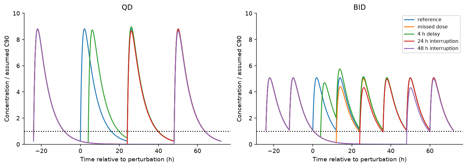
Figure 6. Reference-subject reversible concentrations with a normalized threshold. The schedules are deliberately perturbed mathematical scenarios, not instructions for handling missed medication.
Figure 6 shows that steady-state coverage is not interruption resilience. The expected benefit of regular BID exposure depends on doses actually arriving. More scheduled administrations also creates a different adherence burden, which this PK model does not estimate. These trajectories retain linear PK and do not predict clinical recovery or disease progression.
Saturating absorption
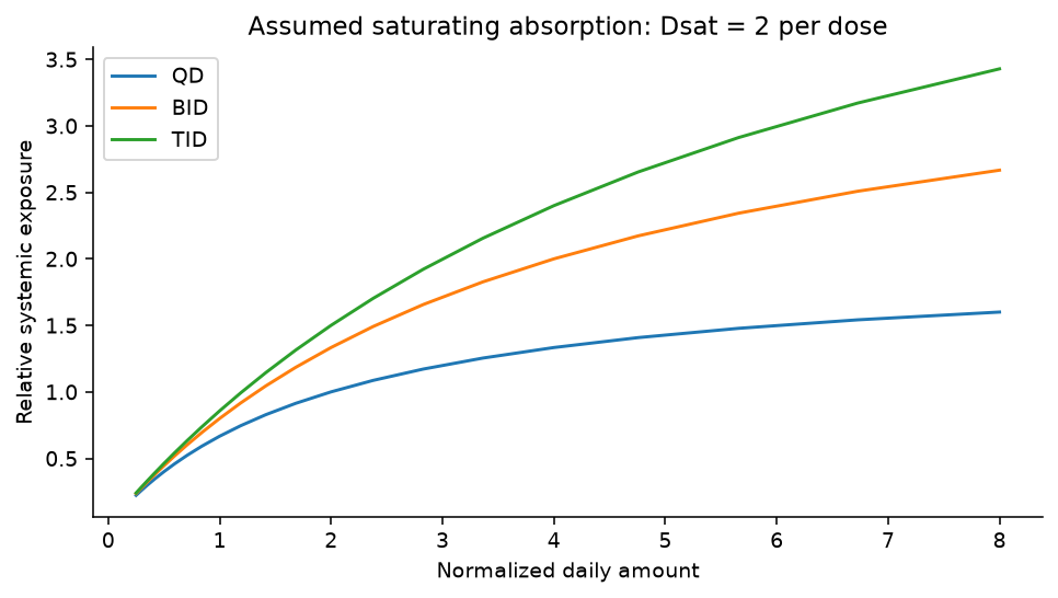
Figure 7. Assumed absorption multiplier \(1/(1+D_{each}/2)\), with normalized amounts. The value 2 is a sensitivity assumption, not a measured RAS inhibitor parameter.
In Figure 7, when exposure is subproportional, splitting the same daily amount can also increase AUC, because each smaller dose has a larger absorbed fraction. The fixed-AUC interpretation of the linear comparison no longer applies. Here local dose elasticity is \(1/(1+D_{each}/2)\). This simple saturating model illustrates why absorption must be checked; it is not fitted to olomorasib or daraxonrasib observations.
Changing clearance
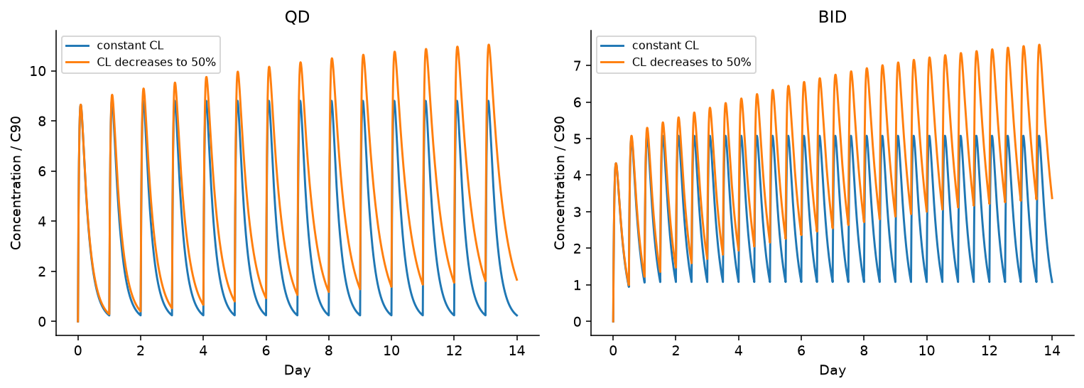
Figure 8. Hypothetical clearance transition half-life 3.5 days. The model is not attributed to a particular compound.
The evolving clearance in Figure 8 invalidates a single stationary profile as a description of every treatment day. Under the assumed decline, later exposures rise even when amount and interval remain unchanged. Time-dependent PK therefore needs repeated observations and a time-aware implementation, rather than copying the terminal half-life into every period.
An exposure–outcome association is not automatically causal
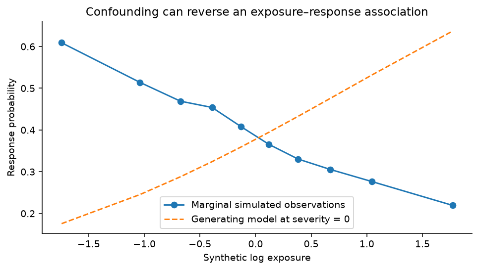
Figure 9. Entirely synthetic data; no clinical patient observations. Higher simulated severity increases exposure and lowers response probability.
For Figure 9, in 20,000 synthetic subjects, I generated log exposure from severity plus noise, then generated response from exposure and severity. The generating exposure log-odds coefficient was +0.6. A naive logistic model estimated −0.506, while the severity-adjusted model estimated +0.575. The example demonstrates a possible sign reversal under explicit assumptions; it does not establish that this mechanism explains any RAS inhibitor trial.
The lesson is methodological: an aggregate exposure–response curve cannot by itself distinguish inadequate drug activity, confounding by illness, changing clearance, selective follow-up, or a true concentration effect. A clinical analysis would require a defensible longitudinal dataset, timing and a specified causal question.
Numerical checks
The periodic analytical PK/tumor solutions agreed with an independent, repeatedly dosed ODE implementation to a maximum absolute error below \(10^{-7}\). High-resolution AUC calculations matched the analytic dose/clearance identity within 0.001%. Exact linear threshold-crossing tests passed. Refining 240 to 960 segments changed reference PTC90 by 0 pp for reversible/covalent models and 0.03 pp for delayed pathway response. Individual TAT differences near the pathway threshold can still reach 4.1 pp; stable population attainment does not prove every trajectory is equally precise.
Discussion
These numerical checks establish implementation consistency. They do not cure the mouse-source unit ambiguity, model residuals, unknown human tumor exposure, unmeasured turnover, assumed population distributions or absence of clinical safety linkage. The Python implementation reconstructs aggregate mouse data and compares hypothetical regimens; it does not estimate human individual variability.
The supported results are public-model reconstruction, identified implementation discrepancies, and paired hypothetical regimen comparisons under specified mechanisms and variability.
These results do not support selecting a clinical QD/BID regimen for a new molecule, deriving a safe starting dose, predicting tumor response, or carrying a mouse pathway threshold directly into a human therapeutic window.
Applying these scenarios to a new molecule requires measurements of human tumor exposure, target or pathway turnover, and between-patient variability. The dose-splitting and interruption comparisons remain conditional on those properties.
Conclusion
Dose splitting changed sustained coverage within the assumed PK/PD and population distributions. Plasma half-life alone did not settle the comparison: distribution, potency, target turnover and exposure variability changed its interpretation. The incomplete mouse reconstruction and unmeasured human properties prevent a clinical regimen recommendation.
Data and code availability
Download the executed notebook, runnable Python code, derived public-data tables, figures and validation results. Run analysis.py, extras.py, then scientific_checks.py; the notebook executes the same calculations. Original source URLs and retrieval status are retained in the source manifest. The bundle contains derived S9 means with attribution; the original supplement can be retrieved separately. All article figures were generated for this analysis.
References
- Jiang J, Jiang L, Maldonato BJ, Wang Y, Holderfield M, Aronchik I, et al. Translational and Therapeutic Evaluation of RAS-GTP Inhibition by RMC-6236 in RAS-Driven Cancers. Cancer Discovery. 2024;14(6):994–1017. doi:10.1158/2159-8290.CD-24-0027. Supplementary Table S8; Supplementary Methods; Supplementary Table S9. Original article and supplements: CC BY 4.0; derived group means retain this attribution.
- Jiang J, Jiang L, Maldonato BJ, Wang Y, Holderfield M, Aronchik I, et al. Correction: Translational and Therapeutic Evaluation of RAS-GTP Inhibition by RMC-6236 in RAS-Driven Cancers. Cancer Discovery. 2025;15(10):2186. doi:10.1158/2159-8290.CD-25-1519.
- Holderfield M, Lee BJ, Jiang J, Tomlinson A, Seamon KJ, Mira A, et al. Concurrent inhibition of oncogenic and wild-type RAS-GTP for cancer therapy. Nature. 2024;629(8013):919–926. doi:10.1038/s41586-024-07205-6.
- Murciano-Goroff YR, Hollebecque A, Heist RS, Cassier PA, Han JY, Kim SY, et al. Pan-tumor activity of olomorasib, a next-generation KRAS G12C inhibitor in KRAS G12C-mutant advanced solid tumors: a first-in-human study. Nature Communications. 2026;17(1):3834. doi:10.1038/s41467-026-69943-7.
- US Food and Drug Administration. RASONQUE (daraxonrasib) prescribing information [Internet]. 2026 [cited 2026 Oct 28]. Section 12.3. Official label.
- Marino S, Hogue IB, Ray CJ, Kirschner DE. A methodology for performing global uncertainty and sensitivity analysis in systems biology. J Theor Biol. 2008;254(1):178–196. doi:10.1016/j.jtbi.2008.04.011.