Before choosing DEG candidates with PIE: average precision versus a follow-up budget
An audit of 10,335 released evaluation rows joins processed DEG labels to average-precision scores. Context-dependent prevalence and paired perturbations clarify what aggregate performance can establish about a limited follow-up budget.
On this page
Background and objective
Predicting which genes change after perturbation could narrow a follow-up experiment. A high AUPRC for differentially expressed gene prediction, however, does not directly tell us how many of the top 50 candidates are correct. In an unfamiliar cellular context, even the number of changing genes differs.
PIE, Perturbation is Everything, predicts population-level expression responses using biological knowledge and observed perturbation data. I joined released evaluation tables associated with its October 5, 2026 preprint to a fixed version of the DEG labels (1). Reaggregating 10,335 evaluation rows separates average performance, DEG scarcity and evaluation under a limited candidate budget.
Predicting population responses
PIE outputs per-gene DEG probabilities, log2 fold changes and mean-expression changes. It predicts a population-level response for a context–perturbation pair rather than matching the future of each individual cell (2).
Inputs include gene descriptions, protein sequences and networks, dependency profiles, cell-line descriptions, control expression and observed perturbation responses from the training set. Using knowledge is not inherently leakage. What matters is which observations remain available when predicting an unseen context. Unseen here means the target context's perturbation responses are excluded from training, not that neither controls nor external knowledge are available (3, 4).
This audit concerns essential-gene CRISPRi data from Replogle–Nadig. It does not establish transfer to drug responses or patient tissues.
Three definitions of unseen conditions
The release contains four folds holding out HepG2, Jurkat, K562 or RPE1. Folder names identify the excluded cell line. The K562 fold was trained and validated on the other three cell lines, not on K562.
Table 1. Reaggregated AUPRC averaged over four folds.
| Setting | Context | Perturbation | Four-fold mean AUPRC |
|---|---|---|---|
| unseen_ctx | Held-out cell line | Present in training | 0.4155 |
| unseen_pert | Three cell lines present in training | Held-out perturbation | 0.3048 |
| unseen_ctx_pert | Held-out cell line | Held-out perturbation | 0.2366 |
These are reaggregations of released scores, not rerun model performance. I first averaged perturbation-level values within context, weighted contexts equally where several were present, and then weighted the four folds equally. Pooling all evaluation rows would use different weights.
I also checked agreement between the 12 evaluation splits and the context and perturbation names in the CSV files. The 10,335 rows represent 5,459 distinct biological context–perturbation pairs, with pairs repeated across folds. Training sets overlap as well. I did not treat rows as independent experiments to construct confidence intervals.
DEG prevalence changes the interpretation of AUPRC
The quantity called true LFC below is an empirically derived reference log2 fold change, not error-free biological truth. Positive labels require a released adjusted p value below 0.05, inclusion among tested genes and a non-NaN reference LFC. In the fixed processed dataset (5), the 5,459×6,642 arrays showed 6,642 tested genes in every row and no NaN reference LFC among them. This traces the processed DEG definition; it does not rerun differential-expression tests from raw counts.
For each pair, define DEG prevalence as:
\[ \pi=\frac{\text{number of DEGs}}{\text{number of tested genes}} \]
An AUPRC has different implications when 1% versus 20% of genes are positive. PIE's binary_auprc implementation computes average precision, AP, which summarizes precision and recall across the ranking. It is distinct from probability calibration and accuracy at a fixed follow-up budget.
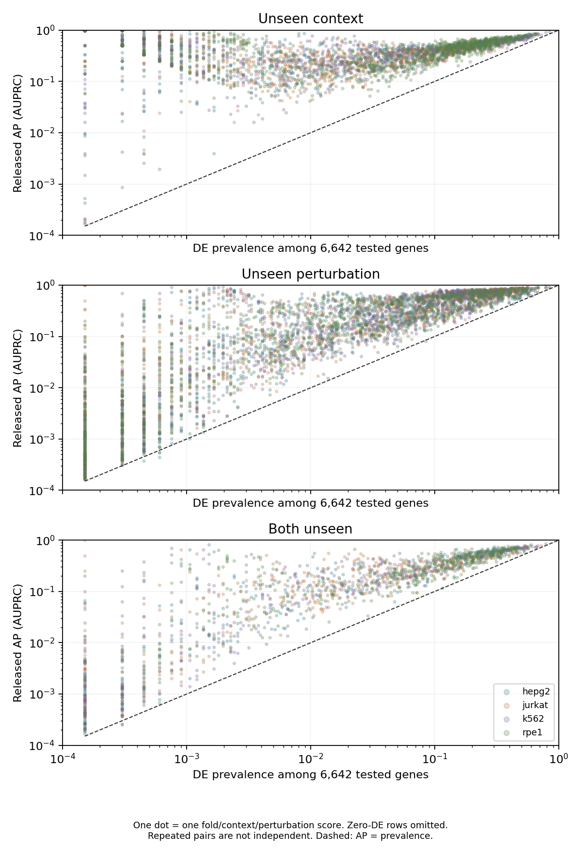
Figure 1. Each point is one fold–context–perturbation evaluation. Color identifies the held-out-context fold, not necessarily the measured context in the central panel. Both axes are logarithmic. The dashed line marks equality between AP and prevalence; it is neither a random-ranking hypothesis test nor a calculation of finite-sample expected AP. Rows with zero DEGs are excluded from the plot.
Prevalence differs substantially across contexts in the jointly unseen setting.
Table 2. DEG prevalence and AP when both context and perturbation are unseen.
| Held-out context | Evaluated pairs | Zero-DEG pairs | Median DEG count | Median prevalence | Mean AP | Median AP/prevalence among nonzero-DEG rows |
|---|---|---|---|---|---|---|
| HepG2 | 386 | 15 | 96.5 | 1.45% | 0.2444 | 3.47 |
| Jurkat | 461 | 3 | 117 | 1.76% | 0.2140 | 5.01 |
| K562 | 430 | 5 | 63 | 0.95% | 0.1984 | 4.54 |
| RPE1 | 470 | 5 | 430.5 | 6.48% | 0.2897 | 3.33 |
RPE1 has a higher mean AP than K562 but also higher DEG prevalence. The median pairwise AP/prevalence ratio reverses that ordering. This ratio is not a new overall score establishing that the K562 model is better. It shows why mean AP alone can hide differences in candidate-selection difficulty.
AP/prevalence is descriptive, not a multiplier of independent follow-up success or a measure of statistical significance. With only one DEG, the small denominator makes the ratio sensitive to a small rank change. The distribution also includes summaries stratifying DEG counts into 0, 1–20, 21–100, 101–500 and above 500.
Zero-DEG rows numbered 48/3,712 for unseen context, 74/4,876 for unseen perturbation and 28/1,747 when both were unseen. The public implementation assigns these rows AP=0 and includes them in means. With no positive labels, AP=0 does not necessarily indicate false-positive predictions. Assessing whether a model can refrain from nominating genes requires false-positive counts or predicted probabilities separately.
Pairing the same unseen perturbations across contexts
I matched perturbations shared between the unseen-perturbation and jointly unseen settings. Within each fold, I averaged AP over available training contexts for each perturbation and subtracted that average from AP in the excluded context. Only matchable perturbations were retained, and the number of known contexts was recorded because some combinations were unmeasured.
Table 3. Paired context differences for the same unseen perturbations.
| Fold | Matched perturbations | Median AP difference: excluded context minus known-context mean | Cases with lower AP in excluded context |
|---|---|---|---|
| HepG2 | 347 | −0.1229 | 303 |
| Jurkat | 416 | −0.0542 | 299 |
| K562 | 371 | −0.0805 | 294 |
| RPE1 | 411 | +0.0317 | 155 |
Three median differences were negative, whereas RPE1's was positive. True DEG counts and biological responses vary across contexts. Matching perturbation names therefore does not causally separate prediction degradation due to an unseen context from biological context differences. The table guards against assuming a uniform proportional decline in every unseen context.
Mean AP does not determine top-50 accuracy
A budget of 50 genes calls for precision@50, recall@50 and an explicit account of conditions in which no candidates are selected. Positives here mean agreement with fixed DEG labels, not successful independent follow-up experiments. Because AP summarizes an entire ranking, equal AP can coexist with different top-ranked accuracy.
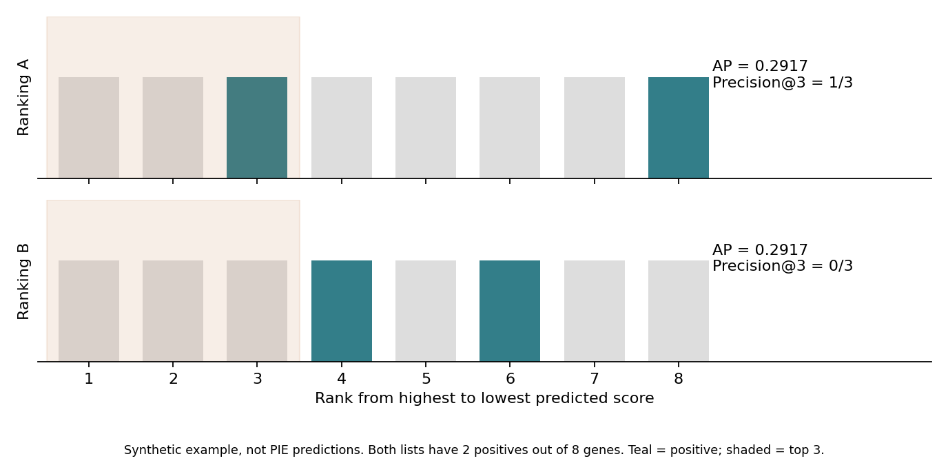
Figure 2. An artificial example, not PIE predictions: eight genes with two positives. Ranking A has positives at positions 3 and 8; ranking B at 4 and 6. Without score ties, both have AP=7/24, approximately 0.2917, but precision among the top three is 1/3 versus 0/3. Their prevalence is also equal.
The pinned model-file inventory contained perturbation-level and context-level evaluation CSVs but no parquet files of per-gene prediction scores. The implementation supports saving predictions, but I did not run checkpoint inference. I therefore did not independently reevaluate PIE precision@50 or source-specific top candidates. Released Jaccard values cannot be converted to precision@50 either.
For comparison, choosing 50 tested genes uniformly without replacement gives:
\[ E[\text{positives}]=50\pi \]
At the median prevalence in the jointly unseen setting, this corresponds to approximately 0.47 positives for K562 and 3.24 for RPE1. These are random-selection expectations, not PIE's observed or guaranteed yield at 50 candidates. Evaluating a ranking at a fixed budget requires the actual ranked scores.
Discussion
PIE combines perturbation knowledge, predicted-gene descriptions, context descriptions and observed response information. The public knowledge card records provenance, model versions and hashes (4).
Even if knowledge-rich perturbations have higher AP, that association would not establish that adding knowledge caused the improvement. Removing a source during training and masking an input only at inference are different interventions. This reaggregation reproduces neither ablation.
Prevalence, zero-DEG frequency and context differences materially affect interpretation of mean AP. They remain separate from evaluating individual ranked candidates at a follow-up budget. Correctly predicting DEGs also does not itself establish disease improvement or avoidance of toxicity.
Data and code availability
Download aggregation code, audit inputs and figures. Audit inputs join released scores to independently extracted DEG counts. Aggregation and nine tests use the Python standard library. Checking against original data requires the download script, numpy and approximately 473 MB of public labels and associated files; figure generation additionally requires matplotlib.
input-provenance.json records model, data, split and implementation revisions and downloaded-file SHA-256 hashes. The distribution excludes checkpoints, embeddings, original evaluation CSVs, label arrays and third-party code. Code licensing (6) and model terms (7) are specified separately.
This is an exploratory audit performed after examining public materials. The original article is a preprint. Primary sources for this audit's numbers and label definitions are the pinned model card, evaluation CSVs, evaluation implementation and processed data. The full paper PDF was unavailable during the audit. I did not verify raw-count differential expression, training or inference, calibration of individual probabilities, top-gene precision, knowledge-source ablations or generalization to patients.
References
- Verma R, Adduri A, Bevilacqua B, Eraslan B, Burke DP, Goodarzi H, et al. PIE: Generalizing perturbation effects across unseen perturbations, contexts and datasets. bioRxiv [Preprint]. Version 1. 2026 Oct 5. doi:10.64898/2026.10.02.756297.
- Arc Institute. PIE: within-dataset generalization on Replogle [Model card and evaluation data]. Revision 055c7a2cabdaff5659121c64fa2b609c231fc5be. Hugging Face. Accessed 2026 Oct 14.
- Arc Institute. PIE [Software]. Commit 21a526add9ff3a81b4f962d9b16bbae570052c63. GitHub. Accessed 2026 Oct 14.
- Arc Institute. PIE: knowledge sources [Dataset card]. Hugging Face. Accessed 2026 Oct 14; retrieved-file hashes recorded in the audit distribution.
- Arc Institute. PIE: Replogle-Nadig essential Perturb-seq [Processed dataset]. Revision 20c9faef76fc96fdc809871340bd93499413dfe7. Hugging Face. Accessed 2026 Oct 14.
- Arc Institute. PIE code license. Commit 21a526add9ff3a81b4f962d9b16bbae570052c63. License.
- Arc Institute. PIE model license. Revision 055c7a2cabdaff5659121c64fa2b609c231fc5be. Model terms.