How was the physiological cliff at menopause reconstructed from data?
A synthetic deconvolution example separates response width from FMP-age variation and examines the timing information supporting menopause reconstruction.
On this page
- Chronological age does not align biological time
- Two populations with different timing information
- Isolating the blurring mechanism
- Different responses can generate the same age mean
- The example does not invalidate the paper’s reconstruction
- Timing information constrains the model
- Data and code availability
- References
“Menopause abruptly changes laboratory measurements throughout the body” might suggest a study following the same people for years. Pridham, Hayut and colleagues instead reconstruct population trajectories relative to the final menstrual period from measurements in people of different ages. Published in Nature Medicine on 12 October 2026, the study was also highlighted on the journal’s X account (1).
The alignment of clocks matters more here than the word “cliff.” At age 50, some people are before their final menstrual period and others after it. Knowing that mixture may help recover a change blurred by chronological-age averaging. I first examine the paper’s methods and then use a synthetic example. The calculation does not estimate actual menopause ages or laboratory trajectories, and it does not rerun YoGlen.
Chronological age does not align biological time
FMP denotes the final menstrual period. Time zero is that period, whereas menopause is confirmed retrospectively after 12 months without menstruation. These are different dates (2). For current age \(a\) and age at FMP \(M\), relative time is
\[ t=a-M \]
At age 50, \(M=47\) means three years after FMP and \(M=53\) means three years before it. Age averages combine both. A sharp change within individuals can therefore appear gradual across an age-ordered population. The same alignment problem arises when onset, treatment initiation or relapse is unrecorded and age or enrollment date substitutes for elapsed time. More measurements do not necessarily repair the clock.
Two populations with different timing information
The paper uses US NHANES and Israeli Clalit data, totaling approximately 300 million tests, not 300 million participants. Longitudinal source records in Clalit do not make the principal reconstruction a directly observed within-person trajectory. The target is a cross-sectional population-mean trajectory aligned to FMP (original Methods).
The authors report significant female–male differences in changes for 52 of 90 tests. Directions vary, and the results include iron and red-cell measures. “Everything deteriorates simultaneously” is not an adequate interpretation (original Fig. 2 and Results).
Table 1. Available timing information and reconstruction methods.
| Data | Information for time alignment | Reconstruction |
|---|---|---|
| NHANES | Age, menstrual status and self-reported FMP age for some participants | Latent FMP ages are multiply imputed; flexible regression models are compared and averaged |
| Clalit | Age-specific laboratory measurements; menstrual status unavailable | A reference FMP-age distribution connects age-specific averages to a piecewise-linear response with a jump and slope change |
NHANES uses 15 imputed datasets and combines uncertainty. Menstrual status constrains whether FMP is before or after the current age; reported FMP provides further information. Ages alone are not used to infer every participant’s clock.
A simplified version of the Clalit model is
\[ f(t)=\beta_0+\alpha_0t+ (\beta_m+\alpha_mt)\mathbf{1}(t>0) \]
This omits additional change points in the original piecewise-linear model. The coefficient \(\beta_m\) represents the FMP jump and \(\alpha_m\) the slope difference. A model capable of a discontinuity is specified before its magnitude is fitted. A corner in the reconstructed curve therefore does not itself establish superiority over arbitrary smooth alternatives. Conversely, allowing a jump does not prove that all results are artifacts. NHANES model selection includes candidates without a jump; cross-population agreement and hormonal comparisons with the longitudinal SWAN study provide additional checks (original YoGlen methods and model selection).
Isolating the blurring mechanism
For the synthetic example, assume everyone shares a mean response \(f(t)\), and FMP age has the same distribution \(p(M)\) regardless of current age. Separate chronological-age effects, birth-cohort differences and selection into care or testing are excluded. Then
\[ g(a)=\int f(a-M)p(M)\,dM \]
The age mean \(g\) averages people at different relative times; reversing that averaging is deconvolution in this setting. The common response is an assumption, not a claim that real individuals follow the same curve. Menstrual status and known FMP ages used by YoGlen are also absent from this example.
Using the standard normal cumulative distribution function \(\Phi\), specify
\[ f(t)=\Phi(t/\tau),\qquad M\sim N(50,\sigma_M^2) \]
The response moves smoothly from zero to one without clinical units. Its scale parameter is \(\tau\); the illustrative normally distributed FMP ages have standard deviation \(\sigma_M\). Integration gives exactly
\[ g(a)=\Phi\!\left( \frac{a-50}{\sqrt{\tau^2+\sigma_M^2}} \right) \]
Thus the observed scale combines response width and variation in FMP age.
Different responses can generate the same age mean
Set \(\tau=1.5\) years and \(\sigma_M=4\) years. The observed scale is
\[ \sqrt{1.5^2+4^2}=\sqrt{18.25}\simeq4.272\ \text{years} \]
The 10–90% transition width is \(2\Phi^{-1}(0.9)\tau\): approximately 3.845 years for the underlying response and 10.950 years for the age average. The 1.5-year scale and 3.845-year transition width are different quantities.
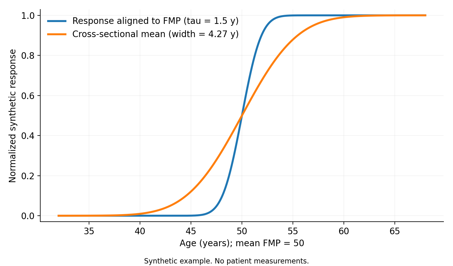
Figure 1. Independent synthetic calculation. Averaging over FMP ages broadens the transition. The unitless response is not measured laboratory data, an estimated clinical transition period or a reproduction of an original figure.
Holding the observed curve fixed while assuming another FMP-age standard deviation gives
\[ \tau_{\mathrm{assumed}}= \sqrt{18.25-\sigma_{M,\mathrm{assumed}}^2} \]
Table 2. Different FMP distributions and response widths yielding the same age average.
| Assumed FMP-age standard deviation | Reconstructed response scale | Response 10–90% width |
|---|---|---|
| 2.0 years | 3.775 years | 9.676 years |
| 3.0 years | 3.041 years | 7.795 years |
| 4.0 years | 1.500 years | 3.845 years |
| 4.2 years | 0.781 years | 2.002 years |
These four combinations generate exactly the same age-mean curve. This is not a small-sample problem. Given only that curve under these assumptions, even zero measurement noise cannot identify the two widths separately.
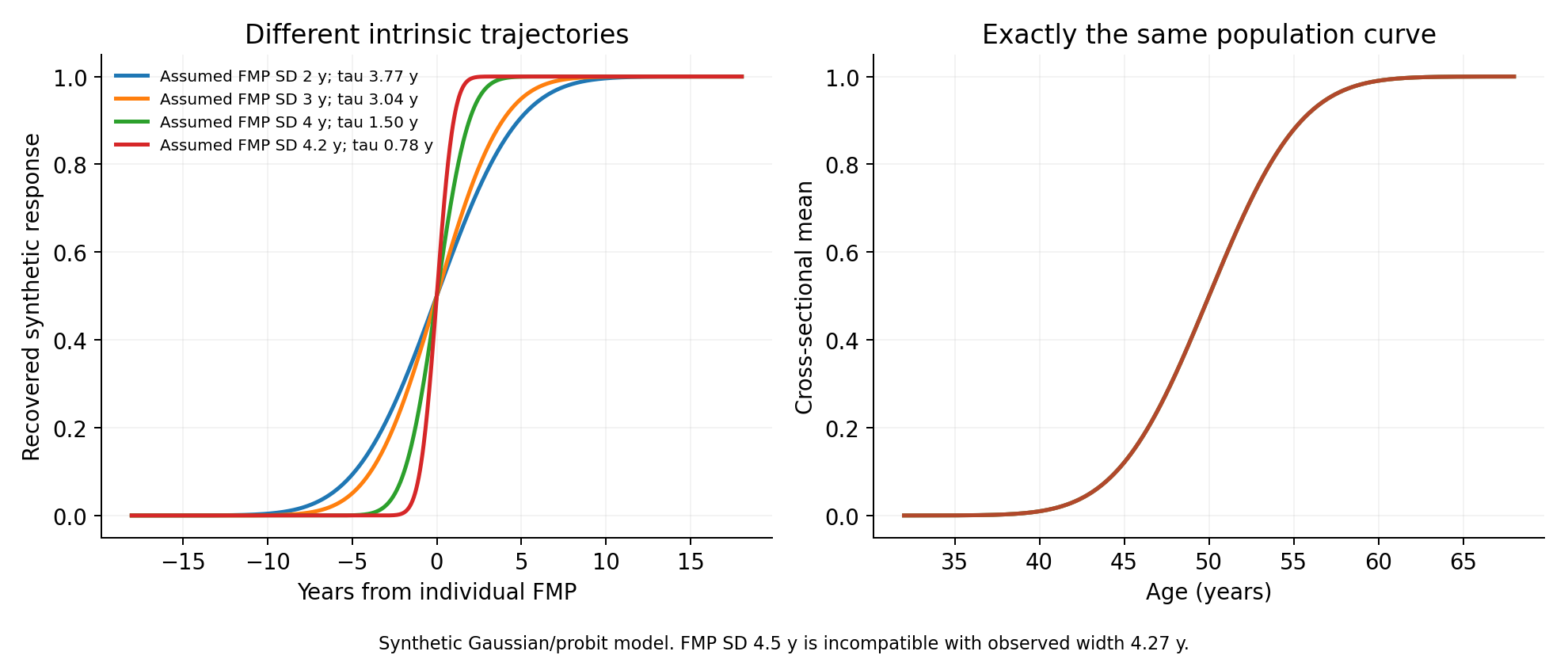
Figure 2. Independent synthetic calculation. The four age-average curves on the right coincide despite different combinations of response and FMP-age widths. This does not reproduce the paper’s sensitivity analysis.
At an assumed FMP-age standard deviation of 4.5 years, the square-root argument is negative. No real response scale explains the observation within this model. Truncating the value to zero and calling the response instantaneous would be incorrect; the assumption and observation are incompatible.
The example does not invalidate the paper’s reconstruction
Menstrual status and reported FMP ages change the information available relative to an age-average-only example. Functional restrictions also reduce freedom. The empirical question is which results remain stable given those restrictions and data.
The authors themselves vary the mean and width of the FMP distribution in simulations. The table above neither establishes nonidentifiability of the entire YoGlen method nor shows an omitted sensitivity analysis (original Extended Data Figs. 1–2). Interpretation instead depends on which timing information is known, which smooth or discontinuous responses the model can express, and sensitivity to FMP distributions, model choices and participant selection. A population mean does not directly become an individual history or forecast.
The jump in original Fig. 2b compares three-year changes in women and men; it is not universally identical to the jump coefficient in the Clalit model. A mathematical discontinuity and a rapid transition over several years are also different claims. Finite measurement frequency makes an exactly zero width difficult to establish, and physiological importance does not require that assertion.
Timing information constrains the model
The paper also reports smaller changes among hormone-therapy users. Background differences between users and nonusers remain possible. Adjusting time and observed covariates alone does not establish treatment benefit or an individual recommendation (original Discussion).
The synthetic calculation constructs different time courses that explain identical observations. A mismatch between the observational clock and the process clock can blur a sharp transition and make its reversal nonunique. The original study constrains this freedom using menstrual information, model structure and comparisons with other populations and longitudinal research. The reconstructed shape depends on independent timing information as well as the number of blood tests.
Data and code availability
The calculation, figures and result CSV files include independently written Python code and execution conditions. They require NumPy, SciPy and Matplotlib. No empirical data are downloaded, YoGlen is not run, and individual FMP ages are not estimated.
python -m pip install -r requirements.txt
python analysis.py
python -m unittest test_analysis.py
python plot.py
Tests compare the exact normal/probit expression against independent numerical integration, verify identical observations from different widths, and detect incompatible width assumptions. All article figures come from this synthetic calculation. Original figures, data and implementation are not bundled. Sources were checked on 18 October 2026. The public YoGlen implementation (3) is linked for reference and is not used in these independent calculations.
References
1. Pridham G, Hayut Y, Lavi-Shoseyov N, Neeman M, Hovav N, Toledano Y, et al. Population-scale reconstruction of menopause dynamics reveals a physiological cliff at the final menstrual period. Nature Medicine. 2026;32:3823–3831. doi:10.1038/s41591-026-04614-0.
2. National Institute on Aging. What is menopause? Health information.
3. Alon Lab. YoGlen. GitHub repository. Source code.